Examples • rmm

I present three examples to demonstrate how the MMMM can be applied to analyze spatial, network, and aggregation problems.

Example 1: The effect of air quality on home values (spatial regression)
Example 2: All friends or just your best friend? (network regression)
Example 3: The effect of political parties’ financial dependency on the survival coalition governments (aggregation regression)

The effect of air quality on home values

The R file of this example can be found here.

This spatial analysis example is based on Harrison & Rubenfield 1978, who study the effect of air quality on home values, and a re-analysis by Bivand 2017.

The study employs census tract data from the Boston Standard Metropolitan Statistical Area in 1970. With tracts containing no housing units or comprised entirely of institutions excluded, the sample contains 506 census tracts. Air quality is measured by the concentration of nitric oxides in the air, which is obtained from a meteorological model (Transportation and Air Shed Simulation Model). I refer to their paper for more information on data and operationalization.

Let us load in the data and plot the home values across town:


library(spData)     # spatial datasets
library(sf)         # read spatial datasets
library(spdep)      # create spatial weights
library(spatialreg) # spatial regression models
library(dplyr)
library(ggplot2)
library(rmm)

# Load spatial data from Boston
boston <- 
  read_sf(system.file("shapes/boston_tracts.gpkg", package = "spData")) %>%
  select(CMEDV, NOX, CRIM, RM, DIS, AGE, LSTAT, geom) %>% 
  st_transform(crs = 5070) %>% # use Albers equal-area conic projection 
  mutate(tid = row_number(), lnCMEDV=log(CMEDV), across(c(NOX, CRIM, RM, DIS, AGE, LSTAT), scale)) %>% 
  relocate(tid, CMEDV, lnCMEDV) 

# Dependent variable:
# lnCMEDV = ln(median home value in $1000)

# Plot median home values across Boston
ggplot(boston, aes(fill = CMEDV)) +
  geom_sf(color = NA) +
  labs(fill = "Median home value") +
  scale_fill_viridis_b() +
  theme(legend.position = "bottom")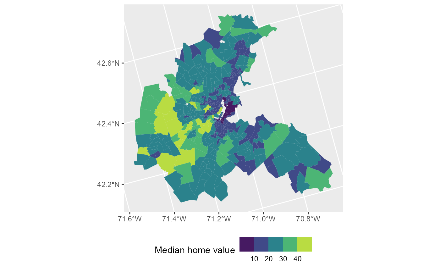


# Explanatory variables (standardized):
# NOX     = nitric oxides concentration 
# CRIM    = per capita crime
# RM      = avg. number of rooms per dwelling
# DIS     = weighted distance to five Boston employment centers
# AGE     = proportion of units built prior 1940 
# LSTAT   = percentage working-class population

First, we examine three canonical spatial regression models:

Residual spatial effect: $Y = XB + \lambda Wu + \epsilon$ . This model is called the spatial error model because it incorporates the residuals of other spatial units into the regression equation of the focal unit.
Exogenous spatial effects: $Y = XB + WXB + \epsilon$ . This model is called the spatial lag-x model because it incorporates the covariates of other spatial units into the regression equation of the focal unit.
Endogenous spatial effect: $Y = \rho WY + XB + \epsilon$ . This model is called the spatial autoregressive model because it incorporates the outcomes of other spatial units into the regression equation of the focal unit.

More information on those models and combinations of them can be found in Gibbons, Overman & Patacchini 2015.

To specify any of these models, we must construct a spatial weight matrix $W$ , which defines the neighborhood structure for each location. $W$ is an $N \times N$ matrix, where $N$ represents the number of neighborhoods. Each element $w_{ij}$ quantifies the relationship between locations $i$ and $j$ , with the convention that $w_{ii} = 0$ along the diagonal.

Neighborhood relationships can be defined in two ways:
- Binary contiguity: $w_{ij} = 1$ if $i$ and $j$ are neighbors, and 0 otherwise.
- Distance-based weighting: $w_{ij}$ is a continuous function of distance.

Continuous weights are often row-standardized so that the sum of all weights for a given location $i$ equals 1.

The R package spatialreg takes the weight matrix as list:

# Create row-standardized weight matrix
boston_nb <- poly2nb(as_Spatial(boston), row.names = boston$tid) # from polygon list to neighbor list

boston_wmat  <- nb2mat(boston_nb, zero.policy = TRUE) %>% as.matrix() # weight matrix
boston_wlist <- nb2listw(boston_nb, style = "W") # weight matrix as list

Now let us estimate the three models:


# Residual spatial effect (spatial error model):
mod1 <- 
  errorsarlm(
    lnCMEDV ~ NOX + CRIM + RM + DIS + AGE,
    data = boston,
    listw = boston_wlist
  )
mod1 %>% summary()
#> 
#> Call:
#> errorsarlm(formula = lnCMEDV ~ NOX + CRIM + RM + DIS + AGE, data = boston, 
#>     listw = boston_wlist)
#> 
#> Residuals:
#>        Min         1Q     Median         3Q        Max 
#> -0.8619402 -0.0727632  0.0019691  0.0727349  0.8610672 
#> 
#> Type: error 
#> Coefficients: (asymptotic standard errors) 
#>               Estimate Std. Error z value  Pr(>|z|)
#> (Intercept)  3.0114297  0.0424386 70.9596 < 2.2e-16
#> NOX         -0.1245513  0.0238428 -5.2238 1.752e-07
#> CRIM        -0.0555031  0.0098813 -5.6170 1.943e-08
#> RM           0.1644857  0.0093976 17.5029 < 2.2e-16
#> DIS         -0.0805092  0.0328909 -2.4478   0.01437
#> AGE         -0.0851376  0.0153088 -5.5613 2.677e-08
#> 
#> Lambda: 0.83765, LR test value: 385.28, p-value: < 2.22e-16
#> Asymptotic standard error: 0.026879
#>     z-value: 31.164, p-value: < 2.22e-16
#> Wald statistic: 971.18, p-value: < 2.22e-16
#> 
#> Log likelihood: 177.6898 for error model
#> ML residual variance (sigma squared): 0.023977, (sigma: 0.15484)
#> Number of observations: 506 
#> Number of parameters estimated: 8 
#> AIC: -339.38, (AIC for lm: 43.904)

# Exogenous spatial effect (spatial lag-x model):  
mod2 <- 
  lmSLX(
    lnCMEDV ~ NOX + CRIM + RM + DIS + AGE,
    data = boston,
    listw = boston_wlist,
    Durbin =  ~ NOX + CRIM + RM + DIS + AGE
  ) 
mod2 %>% summary()
#> 
#> Call:
#> lm(formula = formula(paste("y ~ ", paste(colnames(x)[-1], collapse = "+"))), 
#>     data = as.data.frame(x), weights = weights)
#> 
#> Coefficients:
#>              Estimate    Std. Error  t value     Pr(>|t|)  
#> (Intercept)   3.031e+00   1.043e-02   2.907e+02   0.000e+00
#> NOX          -1.455e-01   4.017e-02  -3.622e+00   3.227e-04
#> CRIM         -5.851e-02   1.503e-02  -3.893e+00   1.125e-04
#> RM            1.538e-01   1.434e-02   1.072e+01   2.856e-24
#> DIS          -6.597e-02   7.453e-02  -8.852e-01   3.765e-01
#> AGE          -9.190e-02   2.369e-02  -3.879e+00   1.190e-04
#> lag.NOX       8.907e-02   4.843e-02   1.839e+00   6.650e-02
#> lag.CRIM     -1.742e-01   2.279e-02  -7.643e+00   1.112e-13
#> lag.RM        8.074e-02   2.211e-02   3.652e+00   2.883e-04
#> lag.DIS      -3.609e-02   7.987e-02  -4.519e-01   6.516e-01
#> lag.AGE       9.673e-03   3.465e-02   2.792e-01   7.802e-01

# Endogenous spatial effect (spatial autoregressive model):
mod3 <- 
  lagsarlm(
    lnCMEDV ~ NOX + CRIM + RM + DIS + AGE,
    data = boston,
    listw = boston_wlist
  )
mod3 %>% summary()
#> 
#> Call:lagsarlm(formula = lnCMEDV ~ NOX + CRIM + RM + DIS + AGE, data = boston, 
#>     listw = boston_wlist)
#> 
#> Residuals:
#>        Min         1Q     Median         3Q        Max 
#> -0.5905925 -0.0937669 -0.0081804  0.0784800  0.9956998 
#> 
#> Type: lag 
#> Coefficients: (asymptotic standard errors) 
#>               Estimate Std. Error z value  Pr(>|z|)
#> (Intercept)  0.9939659  0.0860809 11.5469 < 2.2e-16
#> NOX         -0.0286955  0.0134985 -2.1258 0.0335176
#> CRIM        -0.0606110  0.0087944 -6.8920 5.501e-12
#> RM           0.1343823  0.0088565 15.1732 < 2.2e-16
#> DIS         -0.0627520  0.0132732 -4.7277 2.271e-06
#> AGE         -0.0458586  0.0124080 -3.6959 0.0002191
#> 
#> Rho: 0.67045, LR test value: 347.92, p-value: < 2.22e-16
#> Asymptotic standard error: 0.028312
#>     z-value: 23.681, p-value: < 2.22e-16
#> Wald statistic: 560.8, p-value: < 2.22e-16
#> 
#> Log likelihood: 159.0057 for lag model
#> ML residual variance (sigma squared): 0.028135, (sigma: 0.16774)
#> Number of observations: 506 
#> Number of parameters estimated: 8 
#> AIC: -302.01, (AIC for lm: 43.904)
#> LM test for residual autocorrelation
#> test value: 15.915, p-value: 6.6236e-05

Results:

The spatial error model estimates that after conditioning on those five covariates, the residual is still spatially correlated, as $\lambda$ =0.84.
The spatial lag-x model estimates an exogenous spatial effect for each of the considered covariates. The effect of air quality of neighboring locations, for instance, is estimated to be $\beta$ =0.09. That is, the home values of a given neighborhood increases if the air quality of surrounding neighborhoods decreases.
The spatial autoregessive (SAR) model estimates a endogenous spatial effect of $\rho$ =0.67. That is, the SAR summarizes the spatial dependency in one coefficient.

The MMMM for spatial analysis

Let $y_{i}$ denote the outcome for location $i$ .

Using the MMMM, we can model this outcome based on:
(i) the effects of the location’s own features, $x_{i}^{\intercal} \beta + \epsilon_{i}$
(ii) the effects of its neighbors’ features, $\sum_{j \in n(i)} w_{j} (z_{j}^{\intercal} \gamma + u_{j})$ , where $j$ indexes the neighbors, $n(i)$ is the set of neighbors of location $i$ , $z_{j}$ represents the observed features of neighbor $j$ , and $u_{j}$ captures the combined influence of unobserved features.

This model closely resembles a combination of the spatial lag and spatial error models. The key distinction is that the error term for each location is decomposed into two components: a random effect for its role as a focal location and a separate random effect for its role as a neighbor.

Conceptually, the combination of exogenous spatial effects and spatial error is intuitive, as a location is influenced by its neighbors’ entire right-hand side of the regression equation. In contrast, the endogenous spatial effect model is more challenging to interpret and faces identification issues when both endogenous and exogenous effects are included (spatial Durbin model).

To estimate a spatial MMMM, the neighbors of each location must be included in the dataframe as individual rows:

# Neighbor list to data.frame
nb2df <- function(nb) {
  return(
    data.frame(
      tid = rep(1:length(nb), sapply(nb, length)),
      tid_nb = unlist(nb)
    ) 
  )
}

boston_df <- 
  nb2df(boston_nb) %>% 
  group_by(tid) %>% 
  mutate(n=n()) %>% 
  ungroup() %>% 
  inner_join(boston, by=c("tid")) %>% # own features
  inner_join(                         # neighbor features
    as.data.frame(boston) %>% 
      select(-CMEDV,-lnCMEDV, -geom) %>% 
      rename_with(~paste0(.,"_nb")), 
    by=c("tid_nb")
  )

head(boston_df %>% select(tid, tid_nb, NOX, CRIM, NOX_nb, CRIM_nb))
#> # A tibble: 6 × 6
#>     tid tid_nb NOX[,1] CRIM[,1] NOX_nb[,1] CRIM_nb[,1]
#>   <int>  <int>   <dbl>    <dbl>      <dbl>       <dbl>
#> 1     1      2    1.86    0.624      1.86       0.0275
#> 2     1      3    1.86    0.624      1.86       0.185 
#> 3     1      6    1.86    0.624      1.86       0.0260
#> 4     1      8    1.86    0.624      1.86       0.0708
#> 5     1    311    1.86    0.624      0.434     -0.272 
#> 6     1    313    1.86    0.624      0.434     -0.207

For each tract tid, we have one row for each of its neighbors tid_nb. These rows contain the covariates of tid, which remain constant across its neighbors, as well as the covariates of the neighbors themselves, such as NOX_nb, CRIM_nb, ….

With this setup, we are now ready to estimate the MMMM:


# Spatial random effect:
mod.rmm1 <-
  rmm(
    lnCMEDV ~
      NOX + CRIM + RM + DIS + AGE +
      mm(
        id(tid_nb, tid),
        mmc(),
        mmw(w ~ 1/n, constraint=1)
      ),
    n.iter = 1000, n.burnin = 100, seed=1, monitor = T,
    data = boston_df
  )
#> module glm loaded
#> Compiling model graph
#>    Resolving undeclared variables
#>    Allocating nodes
#> Graph information:
#>    Observed stochastic nodes: 506
#>    Unobserved stochastic nodes: 1020
#>    Total graph size: 20798
#> 
#> Initializing model

names(mod.rmm1)
#> [1] "reg.table" "w"         "re.l1"     "re.l3"     "pred"      "input"    
#> [7] "jags.out"

mod.rmm1 %>% summary()
#>          variable coefficients    sd     lb     ub
#> b.l2[1]        X0        3.035 0.020  2.997  3.075
#> b.l2[2]       NOX       -0.118 0.022 -0.160 -0.075
#> b.l2[3]      CRIM       -0.079 0.010 -0.100 -0.058
#> b.l2[4]        RM        0.170 0.010  0.150  0.190
#> b.l2[5]       DIS       -0.087 0.025 -0.138 -0.038
#> b.l2[6]       AGE       -0.097 0.016 -0.128 -0.065
#> sigma.l1 sigma.l1        0.416 0.023  0.373  0.464
#> sigma.l2 sigma.l2        0.127 0.007  0.113  0.141
#> DIC           DIC      326.073    NA     NA     NA

# Spatial fixed effects + spatial random effect:
mod.rmm2 <-
  rmm(
    lnCMEDV ~
      NOX + CRIM + RM + DIS + AGE +
      mm(
        id(tid_nb, tid),
        mmc(NOX_nb + CRIM_nb + RM_nb + DIS_nb + AGE_nb),
        mmw(w ~ 1/n, constraint=1)
      ),
    n.iter = 1000, n.burnin = 100, seed=1, monitor = T,
    data = boston_df
  )
#> Compiling model graph
#>    Resolving undeclared variables
#>    Allocating nodes
#> Graph information:
#>    Observed stochastic nodes: 506
#>    Unobserved stochastic nodes: 1025
#>    Total graph size: 39277
#> 
#> Initializing model

mod.rmm2 %>% summary()
#>          variable coefficients    sd     lb     ub
#> b.l1[1]    NOX_nb        0.019 0.046 -0.076  0.109
#> b.l1[2]   CRIM_nb       -0.132 0.026 -0.183 -0.079
#> b.l1[3]     RM_nb        0.072 0.025  0.024  0.118
#> b.l1[4]    DIS_nb       -0.013 0.066 -0.142  0.114
#> b.l1[5]    AGE_nb        0.005 0.037 -0.067  0.079
#> b.l2[1]        X0        3.033 0.019  2.996  3.071
#> b.l2[2]       NOX       -0.105 0.029 -0.160 -0.048
#> b.l2[3]      CRIM       -0.061 0.011 -0.081 -0.040
#> b.l2[4]        RM        0.157 0.010  0.138  0.177
#> b.l2[5]       DIS       -0.098 0.056 -0.206  0.012
#> b.l2[6]       AGE       -0.095 0.017 -0.131 -0.061
#> sigma.l1 sigma.l1        0.385 0.024  0.340  0.434
#> sigma.l2 sigma.l2        0.128 0.007  0.115  0.142
#> DIC           DIC      338.542    NA     NA     NA

# Calculate spatial correlation in the residual
getLambda <- function(x) {
  s.l1 <- x$reg.table["sigma.l1", "coefficients"]
  s.l2 <- x$reg.table["sigma.l2", "coefficients"]
  return(s.l1^2/(s.l1^2+s.l2^2))
}

mod.rmm1 %>% getLambda()
#> [1] 0.9153341
mod.rmm2 %>% getLambda()
#> [1] 0.9003032

Let’s take a closer look at thermm() function by typing ?rmm:

The formula object

The most important component is the formula object, which in our case looks like this: lnCMEDV ~ NOX + CRIM + RM + DIS + AGE + mm(id(tid_nb, tid), mmc(NOX_nb + CRIM_nb + RM_nb + DIS_nb + AGE_nb), mmw(w ~ 1/n, constraint=1))

The only difference compared to a lm() formula is the inclusion of the mm() container. Within this container, we define three sub-containers:
- ids() for the identifiers
- mmc() for the covariates being considered,
- mmw() to endogenize the weight function. Here, w ~ 1/n specifies the row-standardized weight.

The combination of the spatial lag and spatial error models can also be estimated within the spatial regression framework. Let’s estimate it and compare the results:


# Exogenous + residual spatial effect (combination of spatial lag model and spatial error model):  
mod2 <- 
  errorsarlm(
    lnCMEDV ~ NOX + CRIM + RM + DIS + AGE,
    data = boston,
    listw = boston_wlist,
    Durbin =  ~ NOX + CRIM + RM + DIS + AGE
  ) 
mod2 %>% summary()
#> 
#> Call:
#> errorsarlm(formula = lnCMEDV ~ NOX + CRIM + RM + DIS + AGE, data = boston, 
#>     listw = boston_wlist, Durbin = ~NOX + CRIM + RM + DIS + AGE)
#> 
#> Residuals:
#>        Min         1Q     Median         3Q        Max 
#> -0.8517313 -0.0713016 -0.0070739  0.0658620  0.8967408 
#> 
#> Type: error 
#> Coefficients: (asymptotic standard errors) 
#>               Estimate Std. Error z value  Pr(>|z|)
#> (Intercept)  3.0149075  0.0331295 91.0037 < 2.2e-16
#> NOX         -0.1120990  0.0244750 -4.5801 4.647e-06
#> CRIM        -0.0667568  0.0100662 -6.6317 3.317e-11
#> RM           0.1687197  0.0094507 17.8526 < 2.2e-16
#> DIS         -0.0863850  0.0423890 -2.0379 0.0415587
#> AGE         -0.0876803  0.0154299 -5.6825 1.328e-08
#> lag.NOX      0.0123545  0.0449974  0.2746 0.7836541
#> lag.CRIM    -0.1031677  0.0269163 -3.8329 0.0001266
#> lag.RM       0.0396613  0.0232693  1.7044 0.0882981
#> lag.DIS     -0.0381250  0.0561561 -0.6789 0.4971937
#> lag.AGE     -0.0196289  0.0380985 -0.5152 0.6064036
#> 
#> Lambda: 0.79294, LR test value: 328.64, p-value: < 2.22e-16
#> Asymptotic standard error: 0.031295
#>     z-value: 25.337, p-value: < 2.22e-16
#> Wald statistic: 641.98, p-value: < 2.22e-16
#> 
#> Log likelihood: 187.0501 for error model
#> ML residual variance (sigma squared): 0.023764, (sigma: 0.15416)
#> Number of observations: 506 
#> Number of parameters estimated: 13 
#> AIC: -348.1, (AIC for lm: -21.461)

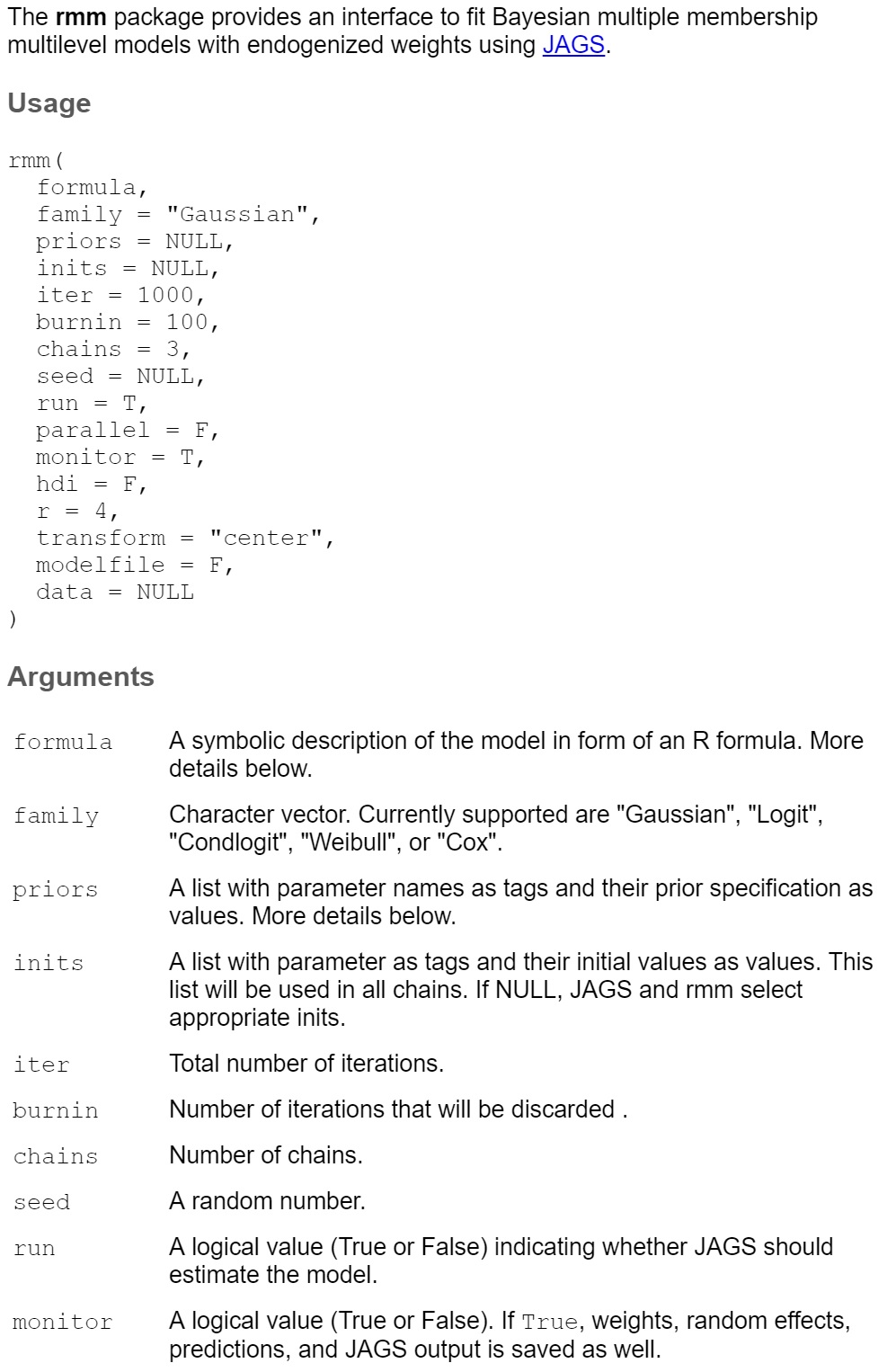
# Plot coefficients next to each other
coefs <- 
  mod.rmm2$reg.table[,c(1,2,4,5)] %>% 
  mutate(model="MMMM") %>% 
  add_row(
    data.frame(model="SLM", coefficients=coef(mod2)[-1], confint(mod2, level=0.95)[-1,]) %>% 
      rename(lb=X2.5.., ub=X97.5..) %>% 
      tibble::rownames_to_column("variable") %>% 
      mutate(
        variable=
          case_when(
            startsWith(variable, "lag.") ~ paste0(sub("lag.", "", variable), "_nb"), 
            variable=="(Intercept)" ~ "X0",
            TRUE ~ variable))
  ) %>% 
  filter(!variable %in% c("X0", "sigma.l1", "sigma.l2", "DIC")) 

ggplot(coefs, aes(x=variable, y=coefficients, color=model)) +
  geom_hline(yintercept = 0, color="red") +
  geom_point(position=position_dodge(width=0.3)) +
  geom_pointrange(aes(ymin = lb, ymax = ub), position=position_dodge(width=0.3))+
  labs(title = "Coefficients", x = "Variables", y="", color="Model") +
  theme(legend.position = "bottom") +
  coord_flip()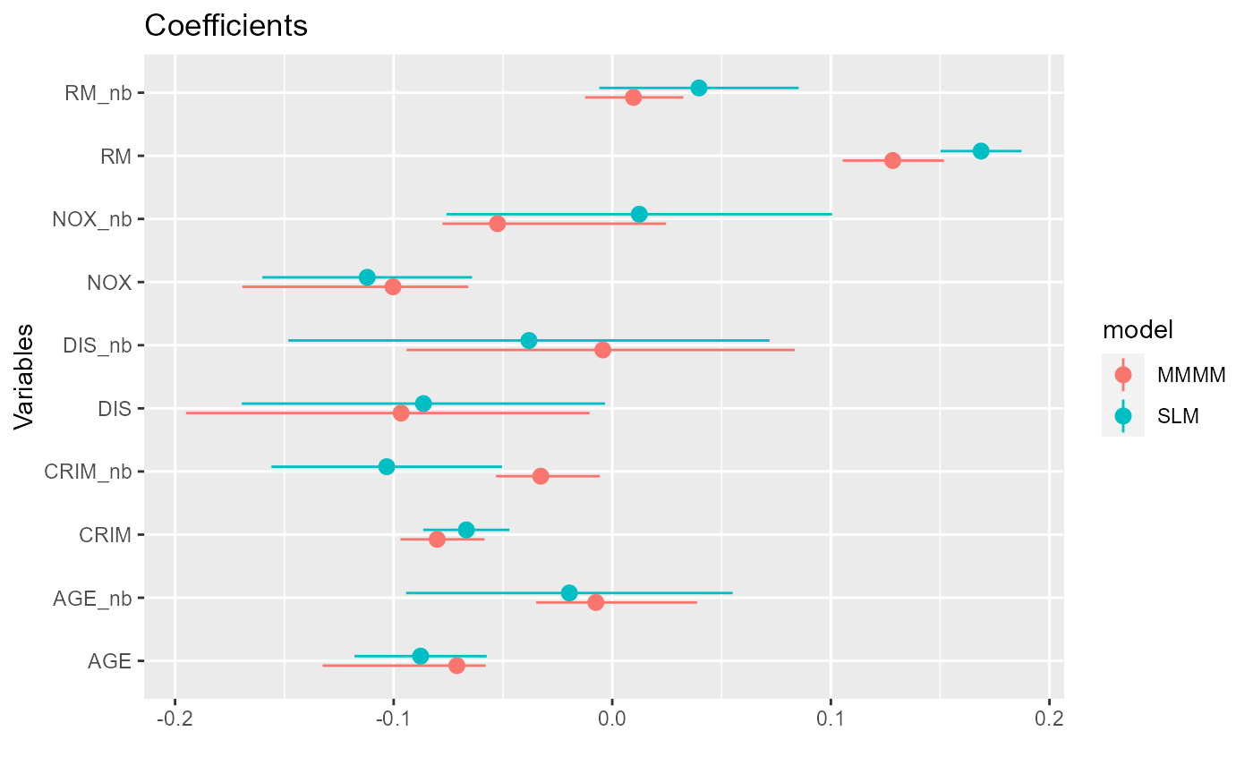

The estimates are similar but not identical due to differences in the estimation algorithms (maximum likelihood vs. Bayesian MCMC) and slight differences in model specifications.

The advantage of using errorsarlm is its faster estimation and ability to account for endogenous errors. If this model aligns with your needs, it is generally best to estimate it using the spatialreg package.

Weight function regression

The MMMM, however, allows the weights to be modeled as a function of covariates. Instead of assuming a fixed weighting scheme, we can estimate whether a neighbor’s influence on a location varies based on specific covariates.

In this example, I hypothesize that a neighbor’s weight in the overall neighborhood effect depends on the similarity between the neighbor and the focal location—an idea inspired by social network theory.

I define similarity as the inverse of the average absolute difference between a neighbor and the focal location across the six considered covariates. This measure captures dissimilarity, so I label the variable DIFF:

# Difference between a focal location and its neighbors
boston_df2 <- 
  boston_df %>% 
  mutate(
    DIFF=1/6*(abs(NOX-NOX_nb)+abs(CRIM-CRIM_nb)+abs(RM-RM_nb)+abs(DIS-DIS_nb)+abs(AGE-AGE_nb)+abs(LSTAT-LSTAT_nb))
  )

The weight function is specified within the mmw() container, allowing for any function that produces bounded weights. Logical operators such as ==, >, < can be used to define conditions that enable aggregation functions, such as min or max.

Here, I use the following functional form:

$w = \frac{1}{n^{\exp(-X\beta)}}$

where $n$ is the number of neighbors of location $i$ , and $X\beta$ represents the covariates used to determine the weights.

This formulation has two key advantages:
1. It ensures weights remain bounded between 0 and 1.
2. When $X\beta = \boldsymbol{0}$ , the weights simplify to $w = \frac{1}{n}$ , which corresponds to the standard row-standardized weights.

The issue of scaling:

With row-standardized weights, the total sum of weights is $\sum_{i=1}^{506} \sum_{j} w_{ij} = \sum_{i=1}^{506} 1 = 506$ .

To ensure this overall sum remains unchanged, we need to carefully specify constraints. Recall that neighbor effects are aggregated as $\sum_{j \in n(i)} w_{j} (z_{j}^{\intercal} \gamma + u_{j})$ .

If the total sum of weights changes, the regression coefficients $\gamma$ will be rescaled. To prevent this, we can apply one of two constraints:

constraint=1: Ensures that the weights of a location’s neighbors sum to 1 for each focal location, while allowing them to vary within each location.
constraint=2: Ensures that all weights sum to the total number of neighborhoods, allowing them to vary both within and across locations.

Both constraints identify the model but have different substantive interpretations. Here, we will use weights that sum to 1 for each focal location while allowing variation within locations (constraint=1):

# Spatial fixed effects + spatial random effect with "endogenized" weights:
mod.rmm3 <-
  rmm(
    lnCMEDV ~
      NOX + CRIM + RM + DIS + AGE +
      mm(
        id(tid_nb, tid),
        mmc(NOX_nb + CRIM_nb + RM_nb + DIS_nb + AGE_nb),
        mmw(w ~ 1/n^exp(-(b1*DIFF)), constraint=1)
      ),
    priors=c("b.w~dnorm(0,1)"), n.iter = 1000, n.burnin = 100, seed=1, monitor = T,
    data = boston_df2
  )
#> Compiling model graph
#>    Resolving undeclared variables
#>    Allocating nodes
#> Graph information:
#>    Observed stochastic nodes: 506
#>    Unobserved stochastic nodes: 1026
#>    Total graph size: 55325
#> 
#> Initializing model

mod.rmm3 %>% summary()
#>          variable coefficients    sd     lb     ub
#> b.l1[1]    NOX_nb        0.001 0.050 -0.099  0.099
#> b.l1[2]   CRIM_nb       -0.161 0.035 -0.228 -0.093
#> b.l1[3]     RM_nb        0.053 0.027 -0.001  0.103
#> b.l1[4]    DIS_nb       -0.064 0.065 -0.191  0.063
#> b.l1[5]    AGE_nb       -0.011 0.037 -0.083  0.061
#> b.l2[1]        X0        3.027 0.018  2.992  3.063
#> b.l2[2]       NOX       -0.067 0.037 -0.141  0.002
#> b.l2[3]      CRIM       -0.044 0.014 -0.071 -0.018
#> b.l2[4]        RM        0.165 0.013  0.139  0.191
#> b.l2[5]       DIS       -0.038 0.055 -0.146  0.064
#> b.l2[6]       AGE       -0.090 0.017 -0.123 -0.058
#> b.w           b.w       -0.969 0.087 -1.152 -0.807
#> sigma.l1 sigma.l1        0.378 0.020  0.342  0.420
#> sigma.l2 sigma.l2        0.099 0.006  0.088  0.111
#> DIC           DIC      355.936    NA     NA     NA

monetPlot(mod.rmm3, parameter="b.w", centrality="median")
#> Registered S3 method overwritten by 'GGally':
#>   method from   
#>   +.gg   ggplot2
#> Warning: package 'patchwork' was built under R version 4.4.2
#> Warning: package 'bayestestR' was built under R version 4.4.2
#> 
#> Attaching package: 'bayestestR'
#> The following object is masked from 'package:ggmcmc':
#> 
#>     ci
#> The following object is masked from 'package:HDInterval':
#> 
#>     hdi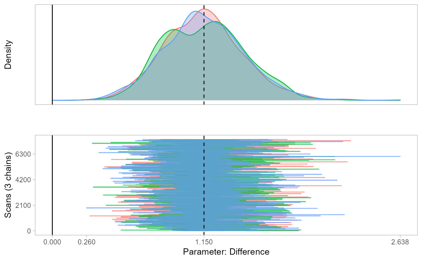

We find that the degree of dissimilarity between a location and its neighbors significantly affects the aggregation weights, with more similar neighbors exerting greater influence than less similar ones.

In other words, features of neighbors that differ significantly from the focal location in terms of air quality, crime levels, and other factors have less impact on home values in the focal neighborhood. This insight would be impossible to uncover using conventional spatial regression models!

If we set monitor=T, we can take a look at the weight estimates:


data.frame(mod.rmm3$w, sum=rowSums(mod.rmm3$w, na.rm = T)) %>% head()
#>                  W1        W2        W3        W4          W5          W6
#> L2 unit 1 0.2135544 0.1831528 0.2588675 0.2059374 0.052230160 0.007778438
#> L2 unit 2 0.1991590 0.2441160 0.2629923 0.2937327          NA          NA
#> L2 unit 3 0.1461061 0.2311961 0.3015582 0.2240084 0.051045581 0.038987162
#> L2 unit 4 0.2513831 0.2783931 0.2206919 0.2495319          NA          NA
#> L2 unit 5 0.2486853 0.2352752 0.2313238 0.1427047 0.007597157 0.005197712
#> L2 unit 6 0.1526319 0.2139220 0.1836577 0.1545417 0.117465724 0.177781097
#>                    W7          W8         W9 W10 W11 W12 W13 W14 W15 sum
#> L2 unit 1 0.003806059 0.074673262         NA  NA  NA  NA  NA  NA  NA   1
#> L2 unit 2          NA          NA         NA  NA  NA  NA  NA  NA  NA   1
#> L2 unit 3 0.004238395 0.002860046         NA  NA  NA  NA  NA  NA  NA   1
#> L2 unit 4          NA          NA         NA  NA  NA  NA  NA  NA  NA   1
#> L2 unit 5 0.084106073 0.029675257 0.01543486  NA  NA  NA  NA  NA  NA   1
#> L2 unit 6          NA          NA         NA  NA  NA  NA  NA  NA  NA   1

rowSums(mod.rmm3$w, na.rm = T) %>% sum()
#> [1] 506

The weights sum to 1 for each focal location but vary across neighbors of each location.

Ben 2do:

Introduce predict() function
Compare predictive performance

All your friends or just your best friend?

A widely used peer effect model in economics is the linear-in-means model, which assumes that all peers in a group exert an equal influence on an individual. In contrast, sociology often emphasizes the best-friend model, which assumes that an individual’s primary influence comes from their closest friend. In this example, I use the MMMM to empirically test which of these models better fits the data.


data(schoolnets)

SAS <- function(nodedat, vars=NULL, suffix) {
  
  # Helper function to select node features as _from or _to
  
  if(is.null(vars)) { # Return all variables if no variable-list specified
    return(
      nodedat %>% 
        dplyr::rename_with(~paste0(., suffix), everything())
    )
  } else {
    return(
      nodedat %>% 
        dplyr::select(!!vars) %>% 
        dplyr::rename_with(~paste0(., suffix), everything())
    )
  }
}

# Create school network data

schoolnets <-
  
  nodedat %>% 
  
  # add friend features
  
  left_join(
    edgedat %>%  
      select(youthid_from, youthid_to, rank) %>% 
      left_join(
        SAS(nodedat, vars=c("youthid", "parent_inc"), suffix="_to"),
        by=c("youthid_to")
      ) %>% 
      group_by(youthid_from) %>%
      mutate(
        bestie = rank==1,
        parent_inc_mean = mean(parent_inc_to, na.rm=T),
      ),
    by=c("youthid"="youthid_from")
  ) %>% 
  
  # count number of friends
  
  tidyr::drop_na() %>% 
  add_count(youthid, name="n_friends") %>% 
  filter(n_friends>=1) %>% 
  
  mutate(across(everything(), ~as.numeric(.)))


# Naive linear-in-means model
mod4 <- lm(test_cogn ~ sex + etn + parent_edu + parent_inc + parent_inc_mean, data=schoolnets) 

# MMMM comparing mean to max aggregation
mod.rmm4 <-
  rmm(
    test_cogn ~
      sex + etn + parent_edu + parent_inc +
      mm(
        id(youthid_to, youthid),
        mmc(parent_inc_to),
        mmw(w ~ b1*1/n_friends+(1-b1)*bestie, constraint=1)
      ),
    n.iter = 1000, n.burnin = 100, seed=1, monitor = T, priors = c("b.w~dunif(0,1)"),
    data = schoolnets
  )
#> Compiling model graph
#>    Resolving undeclared variables
#>    Allocating nodes
#> Graph information:
#>    Observed stochastic nodes: 4814
#>    Unobserved stochastic nodes: 9601
#>    Total graph size: 204654
#> 
#> Initializing model

mod.rmm4 %>% summary()
#>               variable coefficients    sd     lb     ub
#> b.l1     parent_inc_to        0.385 0.049  0.289  0.481
#> b.l2[1]             X0       16.543 0.346 15.878 17.257
#> b.l2[2]            sex        0.166 0.131 -0.101  0.428
#> b.l2[3]            etn       -0.792 0.117 -1.028 -0.569
#> b.l2[4]     parent_edu        0.292 0.077  0.138  0.436
#> b.l2[5]     parent_inc        0.113 0.024  0.067  0.158
#> b.w                b.w        0.967 0.024  0.913  0.998
#> sigma.l1      sigma.l1        3.880 0.132  3.624  4.139
#> sigma.l2      sigma.l2        3.221 0.046  3.133  3.309
#> DIC                DIC    29445.473    NA     NA     NA
monetPlot(mod.rmm4, parameter="b.w", centrality="median") # posterior distribution of the weight coefficient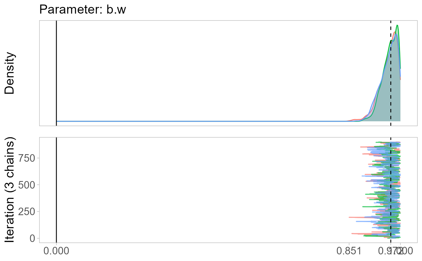


mod.rmm4$w %>% head() # inspect estimated weight matrix
#>                  W1        W2        W3        W4 W5
#> L2 unit 1 0.3551273 0.3224363 0.3224363        NA NA
#> L2 unit 2 0.3551273 0.3224363 0.3224363        NA NA
#> L2 unit 3 0.5163455 0.4836545        NA        NA NA
#> L2 unit 4 0.2745183 0.2418272 0.2418272 0.2418272 NA
#> L2 unit 5 0.2745183 0.2418272 0.2418272 0.2418272 NA
#> L2 unit 6 0.2418272 0.2418272 0.2418272 0.2745183 NA

The results suggest that the linear-in-means model is appropriate: the best friend does not appear to have a greater impact than the other nominated friends as b1=0.97. Since the estimated aggregation is close to linear-in-means, the effect size of parent_inc_to does not differ between models:


coefs <-
  mod.rmm4$reg.table[,c(1,2,4,5)] %>% 
  filter(!variable %in% c("X0", "sigma.l1", "sigma.l2", "DIC")) %>% 
  mutate(model="MMMM") %>% 
  add_row(
    data.frame(model="SLM", coefficients=coef(mod4)[-1], confint(mod4, level=0.95)[-1,]) %>% 
      rename(lb=X2.5.., ub=X97.5..) %>% 
      tibble::rownames_to_column("variable") %>% 
      mutate(variable=ifelse(variable=="parent_inc_mean", "parent_inc_to", variable))
  ) 
rownames(coefs) <- NULL

ggplot(coefs, aes(x=variable, y=coefficients, color=model)) +
  geom_hline(yintercept = 0, color="red") +
  geom_point(position=position_dodge(width=0.3)) +
  geom_pointrange(aes(ymin = lb, ymax = ub), position=position_dodge(width=0.3))+
  labs(title = "Coefficients", x = "Variables", y="", color="Model") +
  theme(legend.position = "bottom") +
  coord_flip()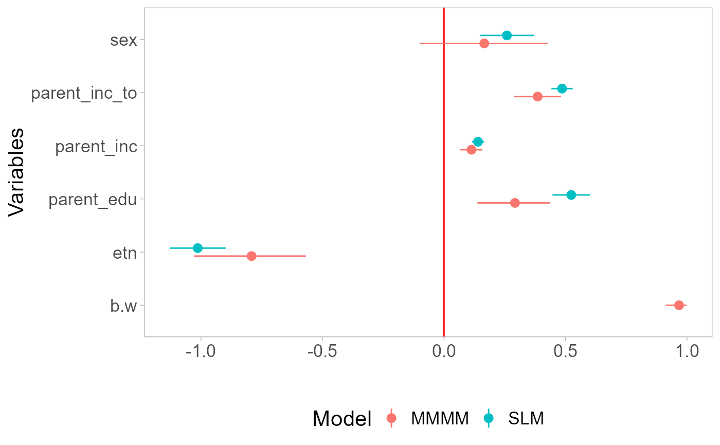

The effect of political parties’ financial dependency on the survival coalition governments

Here, I replicate the example from the paper, examining whether the survival of coalition governments is influenced by parties’ financial dependencies and whether this influence varies across coalition partners. Rosche (2025).

Tbd