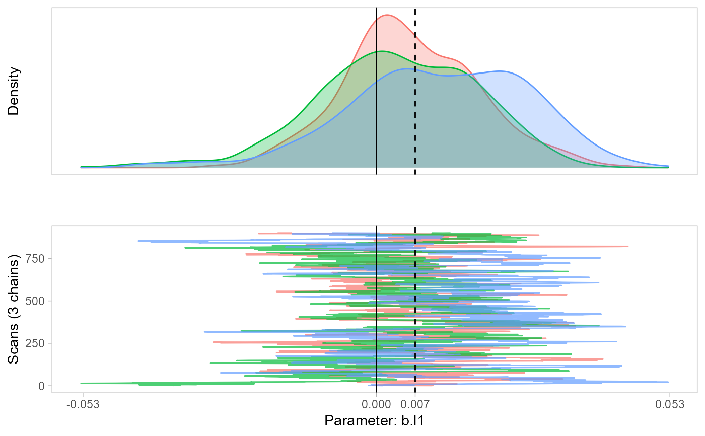
The function monetPlot creates a density plot of the posterior distribution of your model parameters and the traceplot that led to this density.
monetPlot(rmm, parameter, centrality = "median", lab = F, r = 3, sav = F)Arguments
- rmm
A rmm object. rmm has to be run with monitor=T
- parameter
A string with the parameter name. The internal name has to be used, which are the rownames in the rmm reg.table output.
- centrality
A string specifying one of the following options: "median", "mean", "MAP", or "mode".
- lab
String to describe the parameter on the graph's x-axis. Optional. If not specified, the internal parameter name is used.
- r
Specify number of decimal places. Default equals 3.
- sav
TRUE or FALSE (default). If
TRUE, the graph is saved to the current working directory as .png
Value
Returns a plot. The solid vertical is at 0 and the dashed vertical line is the mode of the posterior distributions.
Examples
data(coalgov)
m1 <- rmm(Surv(govdur, earlyterm) ~ 1 + mm(id(pid, gid), mmc(fdep), mmw(w ~ 1/n, constraint=1)) + majority + hm(id=cid, name=cname, type=RE, showFE=F),
          family="Weibull", monitor=T, data=coalgov)
#> module glm loaded
#> Compiling model graph
#>    Resolving undeclared variables
#>    Allocating nodes
#> Graph information:
#>    Observed stochastic nodes: 581
#>    Unobserved stochastic nodes: 843
#>    Total graph size: 14185
#>
#> Initializing model
#>
monetPlot(m1, parameter="b.l1")
#> Registered S3 method overwritten by 'GGally':
#>   method from
#>   +.gg   ggplot2
#> Warning: package 'patchwork' was built under R version 4.4.2
#> Warning: package 'bayestestR' was built under R version 4.4.2
#>
#> Attaching package: 'bayestestR'
#> The following object is masked from 'package:ggmcmc':
#>
#>     ci
#> The following object is masked from 'package:HDInterval':
#>
#>     hdi