Getting Started with ineqx • ineqx

This tutorial walks through the three main workflows of the ineqx package:

Descriptive decomposition — split inequality into within- and between-group components
Causal decomposition — decompose treatment effects on inequality
External GAMLSS model — bring your own model, extract parameters, and decompose

The package has two user-facing functions:

Function	Purpose
`ineqx()`	Variance decomposition — descriptive (no `treat`) or causal (with `treat` or `params`)
`ineqx_params()`	Create parameter object — manually or from a fitted gamlss

We use the simulated incdat dataset that ships with the package. It contains panel data on individuals across multiple years, three groups (group = 1, 2, 3), and a binary treatment indicator (x).

devtools::load_all()
#> ℹ Loading ineqx
#> Warning: package 'testthat' was built under R version 4.5.2

data("incdat")
str(incdat)
#> tibble [3,000 × 7] (S3: tbl_df/tbl/data.frame)
#>  $ id   : int [1:3000] 1 1 2 2 3 3 4 4 5 5 ...
#>  $ year : int [1:3000] 1 1 1 1 1 1 1 1 1 1 ...
#>  $ group: int [1:3000] 1 1 1 1 1 1 1 1 1 1 ...
#>  $ x    : num [1:3000] 0 0 1 1 1 1 1 1 1 1 ...
#>  $ t    : int [1:3000] 0 1 0 1 0 1 0 1 0 1 ...
#>  $ inc  : num [1:3000] 9.88 9.09 8.56 19.2 11.25 ...
#>  $ lninc: num [1:3000] 2.29 2.21 2.15 2.96 2.42 ...

1. Descriptive decomposition

The simplest use case: given an outcome and a grouping variable, how much inequality is within groups versus between groups? When no treat argument is provided, ineqx() performs a descriptive decomposition.

desc <- ineqx(
  y     = "inc",
  group = "group",
  time  = "year",
  ref   = 1,
  ystat = "Var",
  data  = incdat
)
#> Computing descriptive decomposition...
#> Finished.

print(desc)
#> Descriptive variance decomposition
#> Inequality measure: Var 
#> Reference period: 1 
#> Ordering: shapley 
#> 
#> Totals by time:
#>  time   VarW     VarB   VarT
#>     1  40.28  1.23480  41.52
#>     2  59.28  0.03878  59.32
#>     3  90.50  1.83958  92.34
#>     4 136.19  6.49804 142.69
#>     5 192.58 12.92182 205.50
#> 
#> Decomposition of changes in Var relative to ref = 1:
#> 
#>   time 1: (reference)
#> 
#>   time 2:
#>     Between-group (delta_mu):                   -1.1960
#>     Within-group (delta_sigma):                 18.9966
#>     Compositional (delta_pi):                    0.0000
#>       Between-group:                             0.0000
#>       Within-group:                              0.0000
#>     Total:                                      17.8005
#> 
#>   time 3:
#>     Between-group (delta_mu):                    0.6048
#>     Within-group (delta_sigma):                 50.2203
#>     Compositional (delta_pi):                    0.0000
#>       Between-group:                             0.0000
#>       Within-group:                              0.0000
#>     Total:                                      50.8251
#> 
#>   time 4:
#>     Between-group (delta_mu):                    5.2632
#>     Within-group (delta_sigma):                 95.9118
#>     Compositional (delta_pi):                    0.0000
#>       Between-group:                             0.0000
#>       Within-group:                              0.0000
#>     Total:                                     101.1750
#> 
#>   time 5:
#>     Between-group (delta_mu):                   11.6870
#>     Within-group (delta_sigma):                152.2994
#>     Compositional (delta_pi):                    0.0000
#>       Between-group:                             0.0000
#>       Within-group:                              0.0000
#>     Total:                                     163.9864

When a time variable and reference period are provided, ineqx() computes within-group, between-group, and total inequality for each period, and decomposes the change over time into contributions from changing group means ( $\mu$ ), dispersions ( $\sigma$ ), and composition ( $\pi$ ), using Shapley averaging by default.

plot(desc)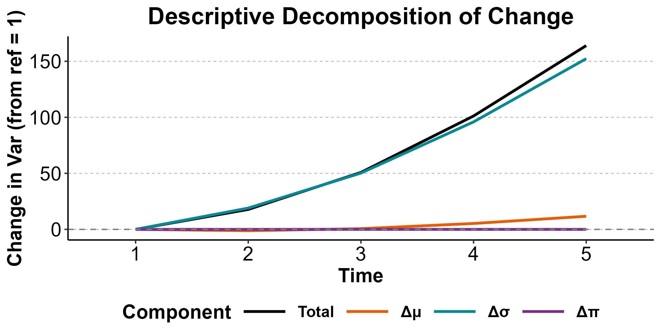

The default plot type is "decomp", which shows how inequality changed relative to the reference period and decomposes that change into $\mu$ , $\sigma$ , and $\pi$ contributions.

Within/between levels

The type = "wibe" plot shows the raw within-group, between-group, and total inequality at each time point:

plot(desc, type = "wibe")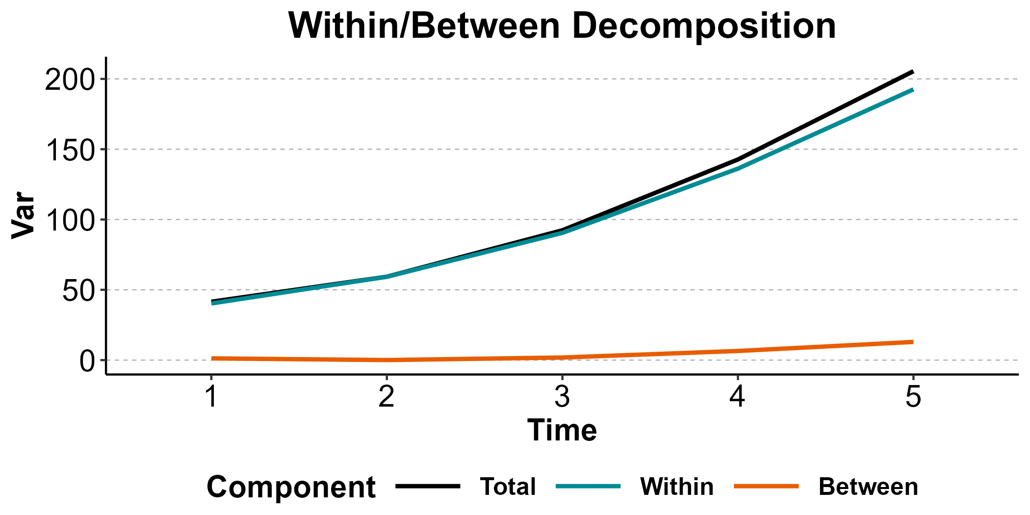

Group-level parameters

The type = "params" plot shows group-level means and standard deviations over time. Pass ci = TRUE or ci = "delta" to add confidence intervals:

plot(desc, type = "params")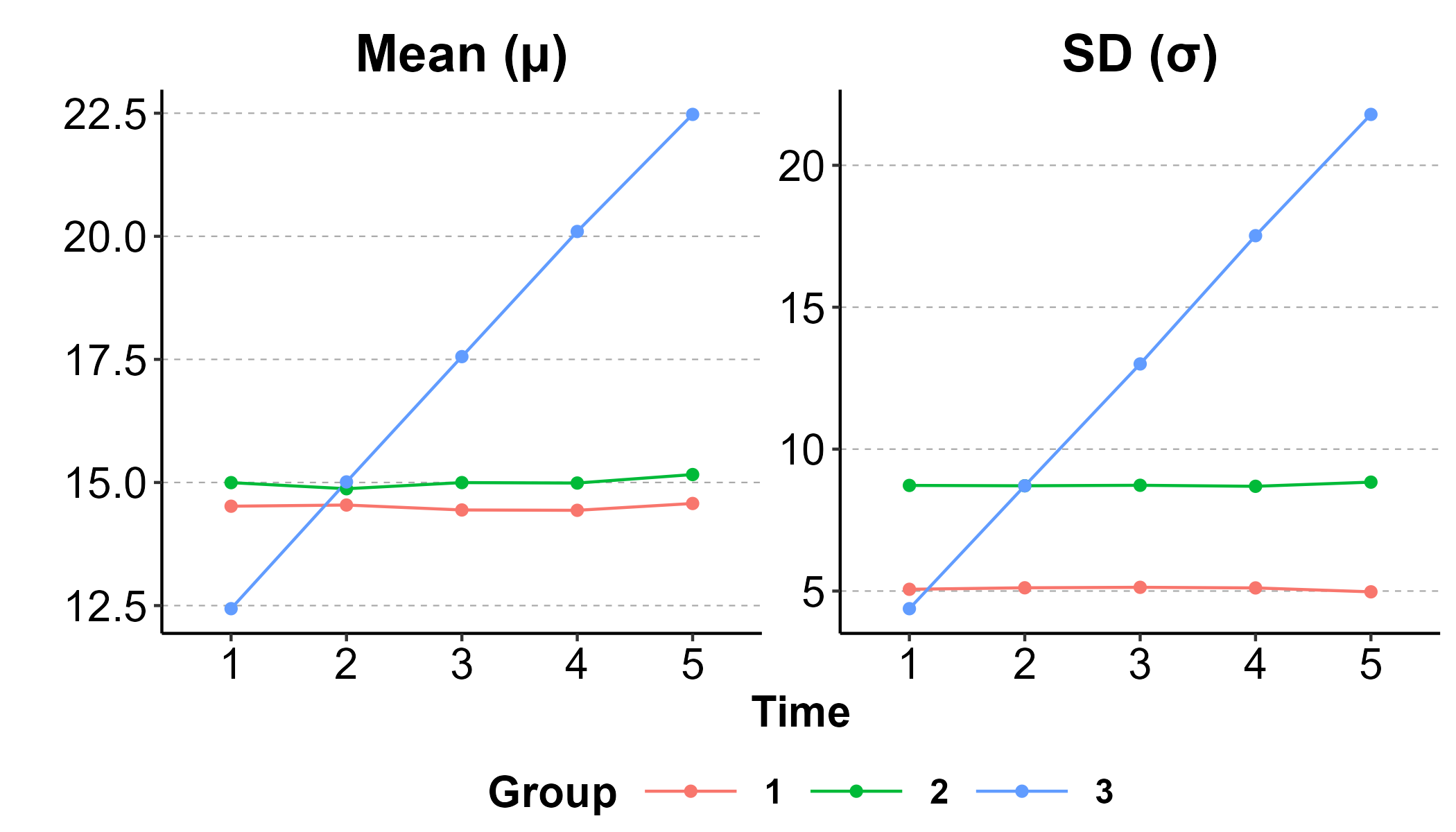

Inequality statistics

The type = "ineq" plot computes and displays overall inequality statistics over time. You can choose from "V" (variance), "VL" (log-variance), "CV2", "Gini", and "Theil", or pass custom functions:

plot(desc, type = "ineq", stats = c("V", "Gini"))

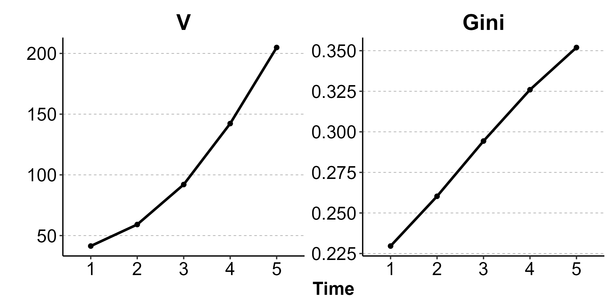
The type = "ineq.group" variant shows per-group inequality statistics:

plot(desc, type = "ineq.group", stats = c("V"))

Counterfactual reference

You can decompose inequality relative to a counterfactual baseline by passing a descriptive params object via params. Create it with ineqx_params() using columns group, pi, mu, sigma — this parallels the causal path where params supplies the reference state.

For example, to decompose the observed inequality into contributions from group means, dispersions, and composition relative to a world of perfect equality (all parameters zero, equal group shares):

ref <- ineqx_params(
  data = data.frame(
    group = 1:3,
    pi    = 1/3,
    mu    = 0,
    sigma = 0
  )
)

desc_ref <- ineqx(
  y     = "inc",
  ystat = "Var",
  group = "group",
  time  = "year",
  params = ref,
  data  = incdat
)
#> Computing descriptive decomposition...
#> Finished.

print(desc_ref)
#> Descriptive variance decomposition
#> Inequality measure: Var 
#> Reference period: 0 
#> Ordering: shapley 
#> 
#> Totals by time:
#>  time   VarW     VarB   VarT
#>     0   0.00  0.00000   0.00
#>     1  40.28  1.23480  41.52
#>     2  59.28  0.03878  59.32
#>     3  90.50  1.83958  92.34
#>     4 136.19  6.49804 142.69
#>     5 192.58 12.92182 205.50
#> 
#> Decomposition of changes in Var relative to counterfactual reference:
#> 
#>   time 0: (reference)
#> 
#>   time 1:
#>     Between-group (delta_mu):                    1.2348
#>     Within-group (delta_sigma):                 40.2821
#>     Compositional (delta_pi):                    0.0000
#>       Between-group:                             0.0000
#>       Within-group:                              0.0000
#>     Total:                                      41.5169
#> 
#>   time 2:
#>     Between-group (delta_mu):                    0.0388
#>     Within-group (delta_sigma):                 59.2786
#>     Compositional (delta_pi):                    0.0000
#>       Between-group:                             0.0000
#>       Within-group:                              0.0000
#>     Total:                                      59.3174
#> 
#>   time 3:
#>     Between-group (delta_mu):                    1.8396
#>     Within-group (delta_sigma):                 90.5024
#>     Compositional (delta_pi):                    0.0000
#>       Between-group:                             0.0000
#>       Within-group:                              0.0000
#>     Total:                                      92.3419
#> 
#>   time 4:
#>     Between-group (delta_mu):                    6.4980
#>     Within-group (delta_sigma):                136.1939
#>     Compositional (delta_pi):                    0.0000
#>       Between-group:                             0.0000
#>       Within-group:                              0.0000
#>     Total:                                     142.6919
#> 
#>   time 5:
#>     Between-group (delta_mu):                   12.9218
#>     Within-group (delta_sigma):                192.5815
#>     Compositional (delta_pi):                    0.0000
#>       Between-group:                             0.0000
#>       Within-group:                              0.0000
#>     Total:                                     205.5033

The deltas show how much each parameter contributes to the level of inequality at each time period: $\mu$ drives between-group inequality, $\sigma$ drives within-group inequality, and $\pi$ captures the effect of unequal group sizes.

2. Causal decomposition

The causal decomposition answers a different question: how does a treatment affect inequality? It decomposes the treatment’s total effect on variance into:

Between-group (behavioral): does treatment raise means more in some groups than others?
Within-group (behavioral): does treatment compress or expand dispersion within groups?

Integrated estimation

The simplest approach: pass formulas and data directly to ineqx(), which fits a GAMLSS model internally. Note that formula_mu is one-sided — the outcome is specified via the y argument:

result <- ineqx(
  y             = "inc",
  treat         = "x",
  group         = "group",
  formula_mu    = ~ x * factor(group),
  formula_sigma = ~ x * factor(group),
  se            = "delta",
  data          = incdat
)
#> GAMLSS-RS iteration 1: Global Deviance = 16642.58 
#> GAMLSS-RS iteration 2: Global Deviance = 16642.58

print(result)
#> Cross-sectional causal variance decomposition
#> Inequality measure: Var 
#> SEs via delta method
#> 
#> Treatment effect on outcome variance:
#>     Var[Y | T = 0]:                          0.9791  (SE = 0.0681)
#>     Var[Y | T = 1]:                        142.4776  (SE = 6.3270)
#>     Total effect (tau_T):                  141.4984  (SE = 6.3274)
#>       Between-group (tau_B):                17.4602  (SE = 2.6803)
#>       Within-group (tau_W):                124.0382  (SE = 5.7317)
#>       -> Wald test H0: lambda = 0: chi2(3) = 7364.6732, p < 0.0001
#>          Significant: evidence of treatment effect heterogeneity
#> 
#> Between-group sub-components:
#>     Var_pi(beta):                           17.6956  (SE = 2.7254)
#>     2*Cov_pi(mu0, beta):                    -0.2354  (SE = 0.3985)
#> 
#> Within-group sub-components:
#>     mean(sigma0^2) * mean(f):              125.6536  (SE = 9.4712)
#>     Cov_pi(sigma0^2, f):                    -1.6154  (SE = 7.4628)

The default type = "wibe" shows the within- and between-group treatment effects as a bar chart. The show argument controls which sub-components to display (default: c("tau", "cov")):

plot(result)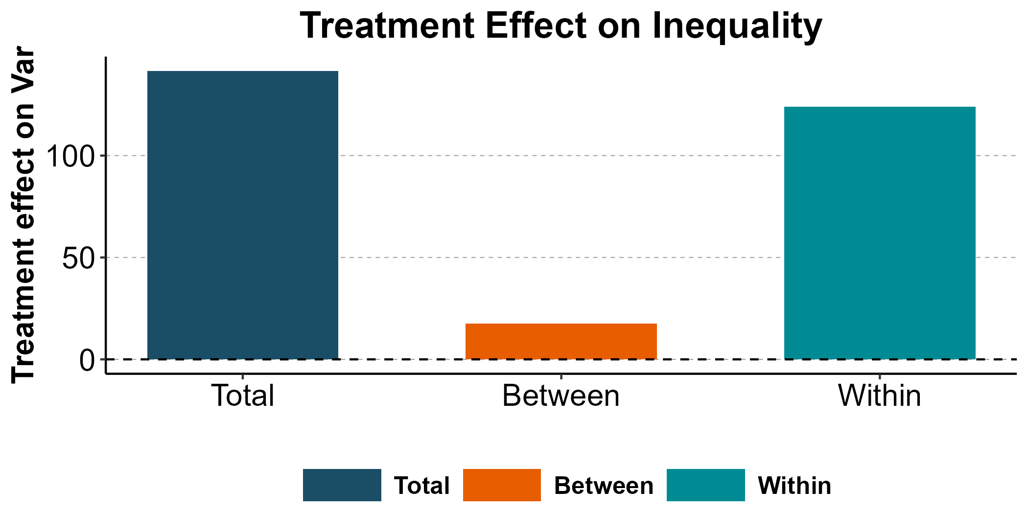

Group-level contributions

The type = "wibe.group" plot shows each group’s contribution to the within-group and between-group treatment effects:

plot(result, type = "wibe.group")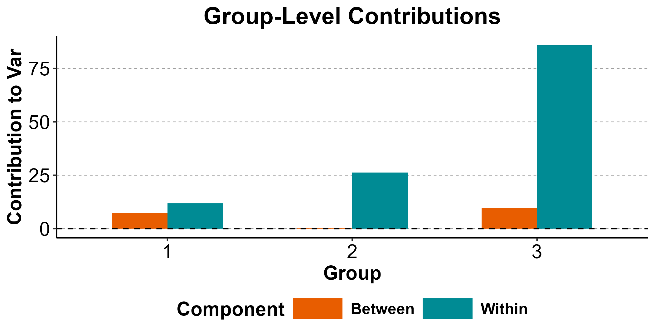

Treatment effect parameters

The type = "treat.params" plot shows the estimated treatment effect parameters ( $\beta$ and $\lambda$ ) by group:

plot(result, type = "treat.params")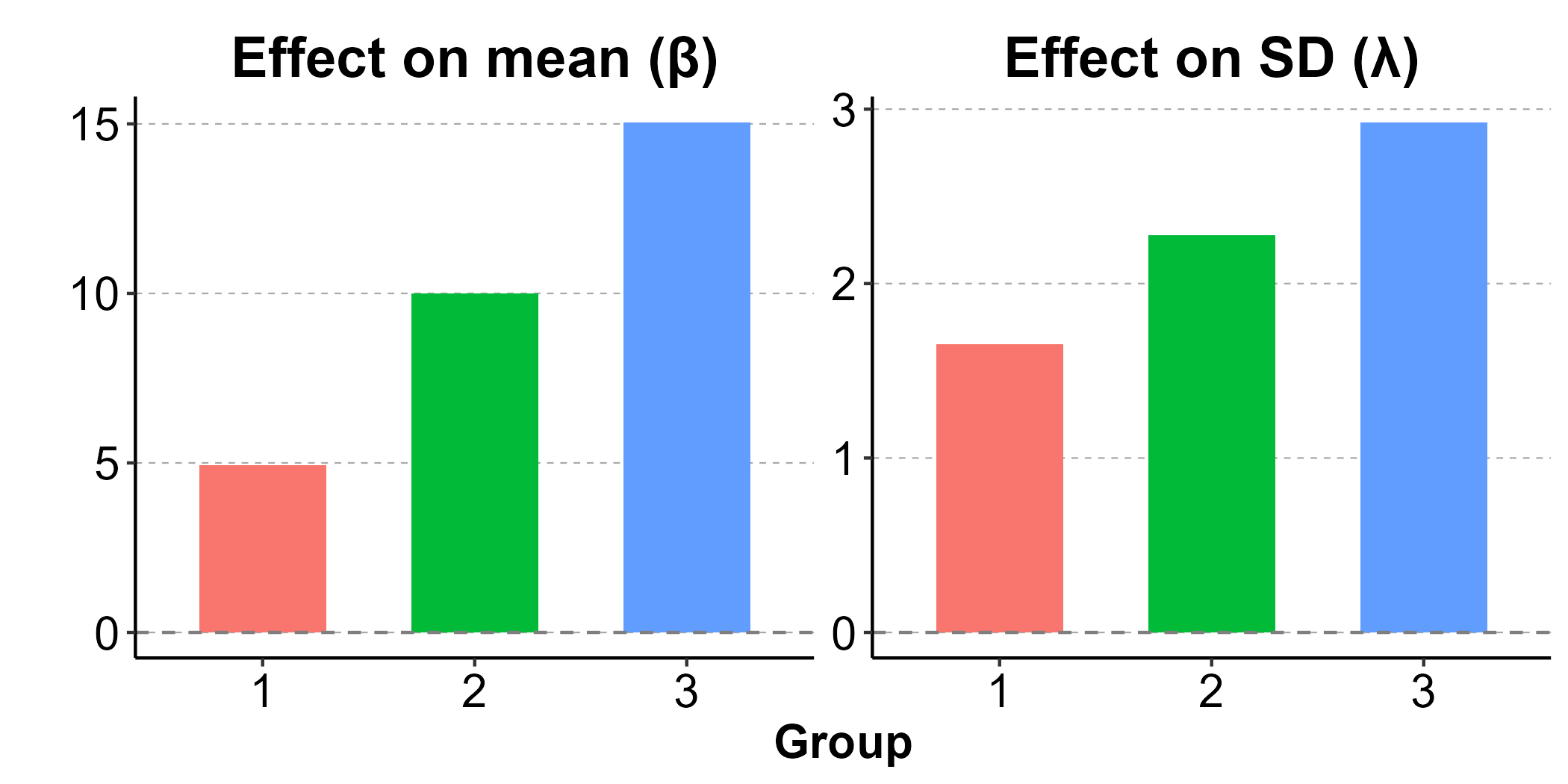

Predicted outcomes

The type = "outcome.params" plot compares predicted group-level means and standard deviations under control versus treatment:

plot(result, type = "outcome.params")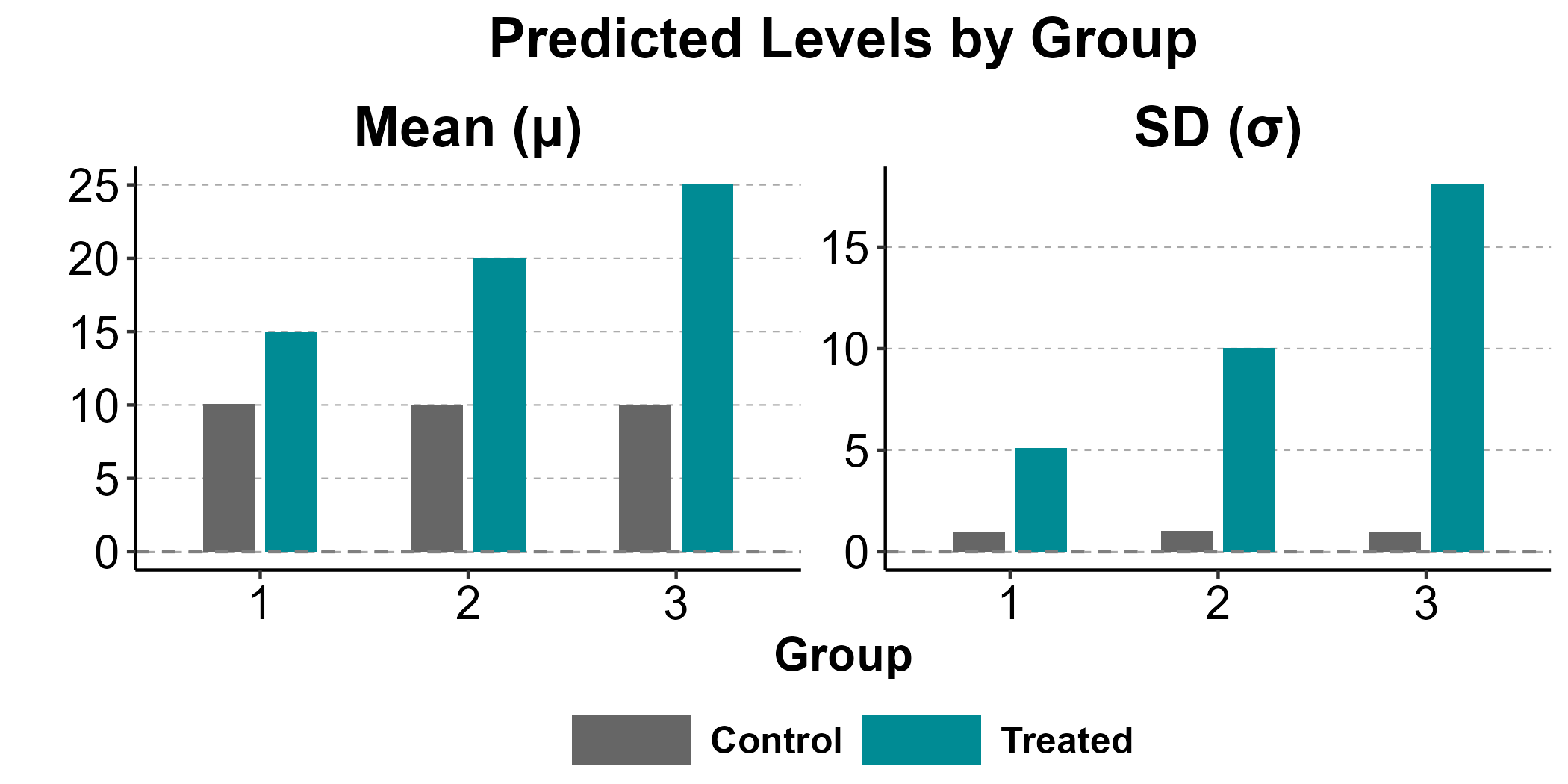

Treatment effect distributions

The type = "treat" plot overlays the predicted treatment effect distributions for each group. Use type = "outcome" to see the full predicted outcome distributions under control vs treatment:

plot(result, type = "treat")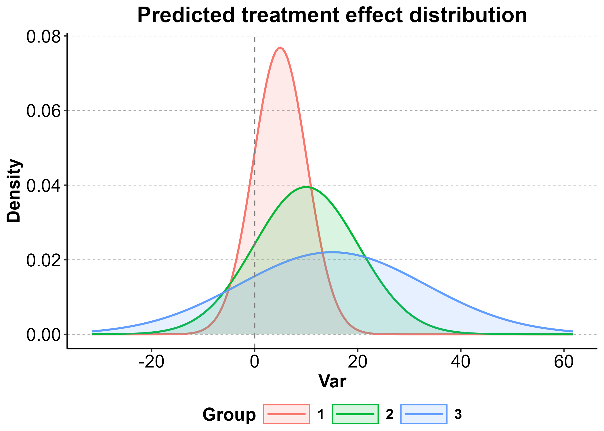

plot(result, type = "outcome")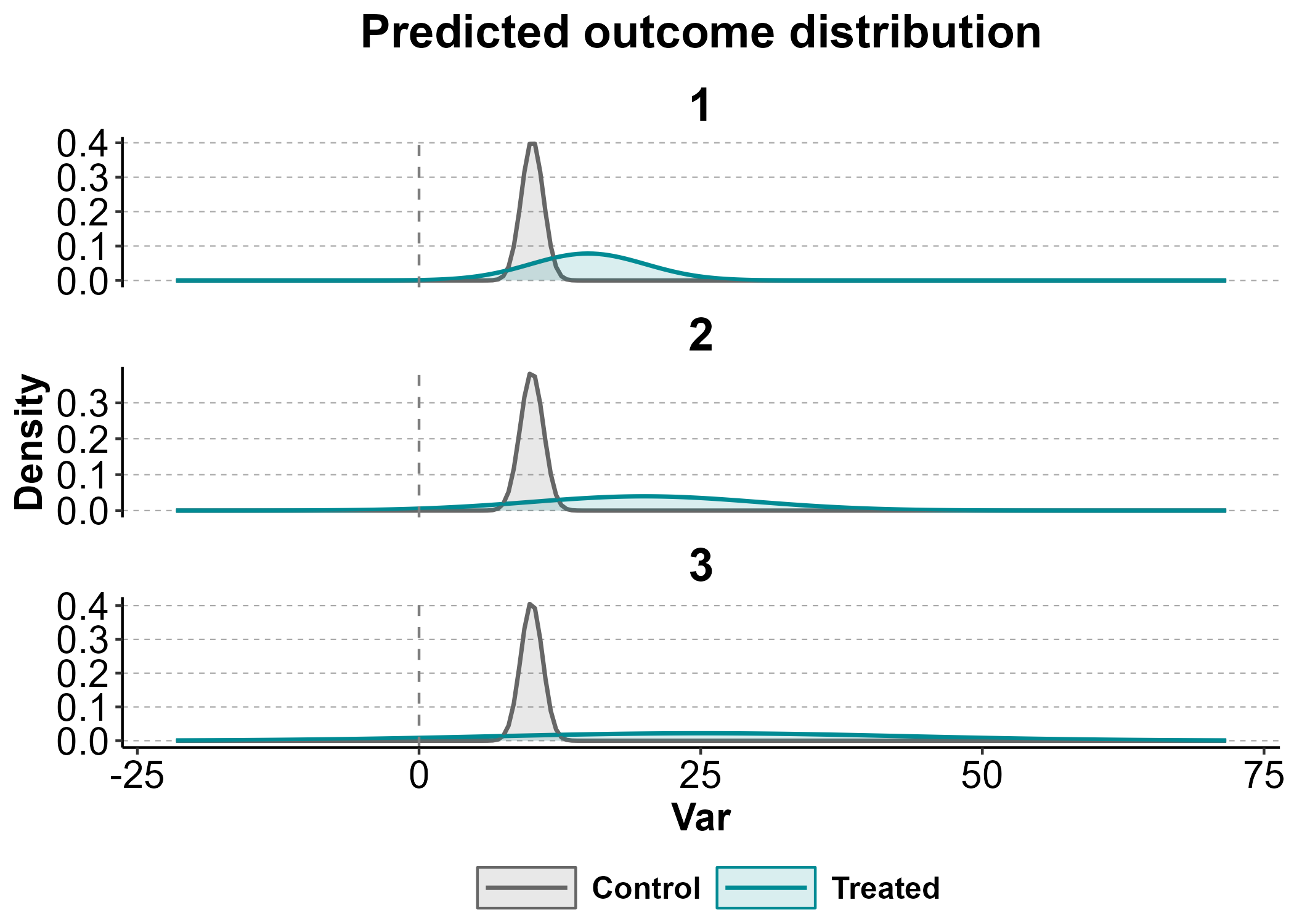

Externally estimated model

For more control, create an ineqx_params object first and pass it to ineqx():

# Extract params from a gamlss model
params <- ineqx_params(
  model = gamlss::gamlss(
    inc ~ x * factor(group) + factor(year),
    sigma.formula = ~ x * factor(group) + factor(year),
    data = incdat, family = gamlss.dist::NO()
  ),
  data  = incdat,
  treat = "x",
  group = "group",
  time  = "year",
  vcov  = TRUE
)
#> GAMLSS-RS iteration 1: Global Deviance = 17539.56 
#> GAMLSS-RS iteration 2: Global Deviance = 16626.77 
#> GAMLSS-RS iteration 3: Global Deviance = 16626.49 
#> GAMLSS-RS iteration 4: Global Deviance = 16626.49

print(params)
#> ineqx_params object
#>   Type: longitudinal 
#>   Inequality measure: Var 
#>   Groups (3): 1, 2, 3
#>   Time periods (5): 1, 2, 3, 4, 5
#> 
#> Group-level parameters:
#> 
#>   time 1:
#>      group     pi    mu0 sigma0   beta lambda
#>          1 0.4737 10.000 0.9100  4.951  1.652
#>          2 0.2632  9.954 0.9620  9.995  2.274
#>          3 0.2632  9.944 0.9028 14.365  2.894
#> 
#>   time 2:
#>      group     pi   mu0 sigma0   beta lambda
#>          1 0.4737 9.966 0.9507  4.951  1.652
#>          2 0.2632 9.920 1.0050  9.995  2.274
#>          3 0.2632 9.911 0.9431 14.365  2.894
#> 
#>   time 3:
#>      group     pi   mu0 sigma0   beta lambda
#>          1 0.4737 10.10 0.9916  4.951  1.652
#>          2 0.2632 10.05 1.0482  9.995  2.274
#>          3 0.2632 10.05 0.9837 14.365  2.894
#> 
#>   time 4:
#>      group     pi   mu0 sigma0   beta lambda
#>          1 0.4737 10.08 1.0018  4.951  1.652
#>          2 0.2632 10.04 1.0591  9.995  2.274
#>          3 0.2632 10.03 0.9939 14.365  2.894
#> 
#>   time 5:
#>      group     pi   mu0 sigma0   beta lambda
#>          1 0.4737 10.10  1.051  4.951  1.652
#>          2 0.2632 10.06  1.111  9.995  2.274
#>          3 0.2632 10.05  1.042 14.365  2.894
#> 
#> vcov: 5 time periods

Longitudinal causal decomposition

With longitudinal parameters, ineqx() automatically performs the longitudinal decomposition:

result_longit <- ineqx(
  "inc",
  group  = "group",
  ref    = 1,
  order  = c("behavioral", "compositional", "pretreatment"),
  params = params,
  se     = "delta",
  data   = incdat
)
#> Computing decomposition...
#> Finished.

print(result_longit)
#> Longitudinal causal variance decomposition
#> Inequality measure: Var 
#> SEs via delta method
#> Reference period: 1 
#> Ordering: behavioral -> compositional -> pretreatment 
#> 
#> Treatment effect on variance by time:
#> (tau_B = Var(beta) + 2Cov(mu,beta);  tau_W = E(sigma^2)*E(f) + Cov(sigma^2,f);  tau_T = tau_B + tau_W)
#> 
#>  time  Var(beta)  2Cov(mu,beta)      tau_B E(sigma2)*E(f)  Cov(sigma2,f)      tau_W      tau_T   lambda=0 
#>     1    15.5392        -0.1934    15.3459       104.1931        -1.4450   102.7481   118.0939     <0.001 
#>    SE   (2.4384)       (0.3789)   (2.3962)       (9.4268)       (6.0948)   (7.0774)   (7.4720)            
#>     2    15.5392        -0.1934    15.3459       113.7054        -1.5770   112.1285   127.4743     <0.001 
#>    SE   (2.4384)       (0.3789)   (2.3962)      (10.2875)       (6.6513)   (7.7235)   (8.0867)            
#>     3    15.5392        -0.1934    15.3459       123.7010        -1.7156   121.9854   137.3313     <0.001 
#>    SE   (2.4384)       (0.3789)   (2.3962)      (11.1918)       (7.2360)   (8.4024)   (8.7374)            
#>     4    15.5392        -0.1934    15.3459       126.2725        -1.7512   124.5213   139.8671     <0.001 
#>    SE   (2.4384)       (0.3789)   (2.3962)      (11.4245)       (7.3864)   (8.5771)   (8.9055)            
#>     5    15.5392        -0.1934    15.3459       138.8845        -1.9262   136.9583   152.3042     <0.001 
#>    SE   (2.4384)       (0.3789)   (2.3962)      (12.5655)       (8.1241)   (9.4338)   (9.7334)            
#> 
#> Decomposition of changes in group-specific treatment effects on variance relative to ref = 1:
#> 
#>   time 1: (reference)
#> 
#>   time 2:
#>     Effects on means (delta_beta):                       0.0000  (SE = 3.4297)
#>     Effects on SDs (delta_lambda):                       0.0000  (SE = 9.5802)
#>     Distribution of treatment (delta_pi):                0.0000  (SE = 0.0000)
#>       Between-group:                                     0.0000
#>       Within-group:                                      0.0000
#>     Pre-treatment inequality (delta_pre):                9.3804  (SE = 10.4581)
#>       Means:                                             0.0000
#>       Variances:                                         9.3804
#>     Total:                                               9.3804  (SE = 11.0102)
#> 
#>   time 3:
#>     Effects on means (delta_beta):                       0.0000  (SE = 3.4297)
#>     Effects on SDs (delta_lambda):                      -0.0000  (SE = 9.5802)
#>     Distribution of treatment (delta_pi):                0.0000  (SE = 0.0000)
#>       Between-group:                                     0.0000
#>       Within-group:                                      0.0000
#>     Pre-treatment inequality (delta_pre):               19.2373  (SE = 10.7741)
#>       Means:                                             0.0000
#>       Variances:                                        19.2373
#>     Total:                                              19.2373  (SE = 11.4967)
#> 
#>   time 4:
#>     Effects on means (delta_beta):                      -0.0000  (SE = 3.4297)
#>     Effects on SDs (delta_lambda):                       0.0000  (SE = 9.5802)
#>     Distribution of treatment (delta_pi):                0.0000  (SE = 0.0000)
#>       Between-group:                                     0.0000
#>       Within-group:                                      0.0000
#>     Pre-treatment inequality (delta_pre):               21.7732  (SE = 10.8608)
#>       Means:                                             0.0000
#>       Variances:                                        21.7732
#>     Total:                                              21.7732  (SE = 11.6250)
#> 
#>   time 5:
#>     Effects on means (delta_beta):                      -0.0000  (SE = 3.4297)
#>     Effects on SDs (delta_lambda):                      -0.0000  (SE = 9.5802)
#>     Distribution of treatment (delta_pi):                0.0000  (SE = 0.0000)
#>       Between-group:                                     0.0000
#>       Within-group:                                      0.0000
#>     Pre-treatment inequality (delta_pre):               34.2102  (SE = 11.3153)
#>       Means:                                            -0.0000
#>       Variances:                                        34.2102
#>     Total:                                              34.2102  (SE = 12.2707)

The default type = "decomp" shows the three-component decomposition (behavioral, compositional, pre-treatment) of changes relative to the reference:

plot(result_longit)

Six sub-component decomposition

Setting show to individual delta components displays the six sub-components ( $\Delta_\beta$ , $\Delta_\lambda$ , $\Delta_{\pi,b}$ , $\Delta_{\pi,w}$ , $\Delta_\mu$ , $\Delta_\sigma$ ):

plot(result_longit, type = "decomp",
     show = c("delta_beta", "delta_lambda", "delta_pi_b",
              "delta_pi_w", "delta_mu", "delta_sigma"))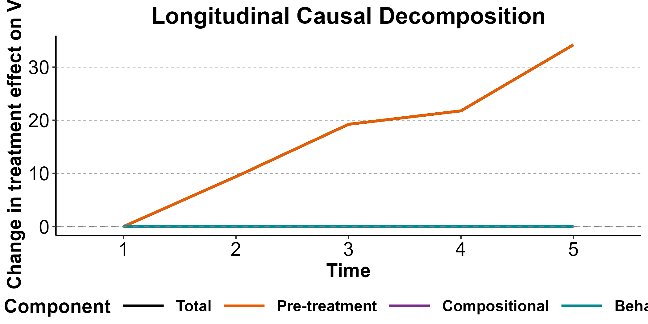

Within- and between-group treatment effects

The type = "wibe" plot shows the levels of the cross-sectional treatment effects ( $\tau_B$ , $\tau_W$ ) at each time point, rather than changes from the reference. The show argument controls which sub-components to display (default: c("tau_b", "tau_w"); also available: "het_b", "cov_b", "het_w", "cov_w"):

plot(result_longit, type = "wibe")

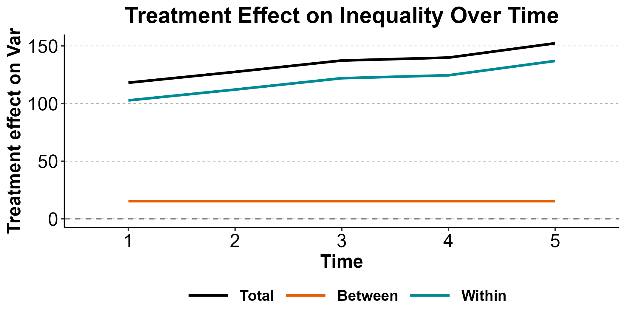
Shapley values

Since the longitudinal decomposition depends on the ordering, you can average across all 6 orderings with order = "shapley":

result_shapley <- ineqx("inc", group = "group", ref = 1,
                         params = params, order = "shapley",
                         se = "none", data = incdat)
#> Computing decomposition...
#> Finished.
print(result_shapley)
#> Longitudinal causal variance decomposition
#> Inequality measure: Var 
#> Reference period: 1 
#> Ordering: Shapley (averaged across all 6 orderings)
#> 
#> Treatment effect on variance by time:
#> (tau_B = Var(beta) + 2Cov(mu,beta);  tau_W = E(sigma^2)*E(f) + Cov(sigma^2,f);  tau_T = tau_B + tau_W)
#> 
#>  time  Var(beta)  2Cov(mu,beta)      tau_B E(sigma2)*E(f)  Cov(sigma2,f)      tau_W      tau_T 
#>     1    15.5392        -0.1934    15.3459       104.1931        -1.4450   102.7481   118.0939 
#>     2    15.5392        -0.1934    15.3459       113.7054        -1.5770   112.1285   127.4743 
#>     3    15.5392        -0.1934    15.3459       123.7010        -1.7156   121.9854   137.3313 
#>     4    15.5392        -0.1934    15.3459       126.2725        -1.7512   124.5213   139.8671 
#>     5    15.5392        -0.1934    15.3459       138.8845        -1.9262   136.9583   152.3042 
#> 
#> Decomposition of changes in group-specific treatment effects on variance relative to ref = 1:
#> 
#>   time 1: (reference)
#> 
#>   time 2:
#>     Effects on means (delta_beta):                       0.0000
#>     Effects on SDs (delta_lambda):                       0.0000
#>     Distribution of treatment (delta_pi):                0.0000
#>       Between-group:                                     0.0000
#>       Within-group:                                      0.0000
#>     Pre-treatment inequality (delta_pre):                9.3804
#>       Means:                                             0.0000
#>       Variances:                                         9.3804
#>     Total:                                               9.3804
#> 
#>   time 3:
#>     Effects on means (delta_beta):                       0.0000
#>     Effects on SDs (delta_lambda):                      -0.0000
#>     Distribution of treatment (delta_pi):                0.0000
#>       Between-group:                                     0.0000
#>       Within-group:                                      0.0000
#>     Pre-treatment inequality (delta_pre):               19.2373
#>       Means:                                             0.0000
#>       Variances:                                        19.2373
#>     Total:                                              19.2373
#> 
#>   time 4:
#>     Effects on means (delta_beta):                      -0.0000
#>     Effects on SDs (delta_lambda):                       0.0000
#>     Distribution of treatment (delta_pi):                0.0000
#>       Between-group:                                     0.0000
#>       Within-group:                                      0.0000
#>     Pre-treatment inequality (delta_pre):               21.7732
#>       Means:                                             0.0000
#>       Variances:                                        21.7732
#>     Total:                                              21.7732
#> 
#>   time 5:
#>     Effects on means (delta_beta):                      -0.0000
#>     Effects on SDs (delta_lambda):                      -0.0000
#>     Distribution of treatment (delta_pi):                0.0000
#>       Between-group:                                     0.0000
#>       Within-group:                                      0.0000
#>     Pre-treatment inequality (delta_pre):               34.2102
#>       Means:                                            -0.0000
#>       Variances:                                        34.2102
#>     Total:                                              34.2102

plot(result_shapley)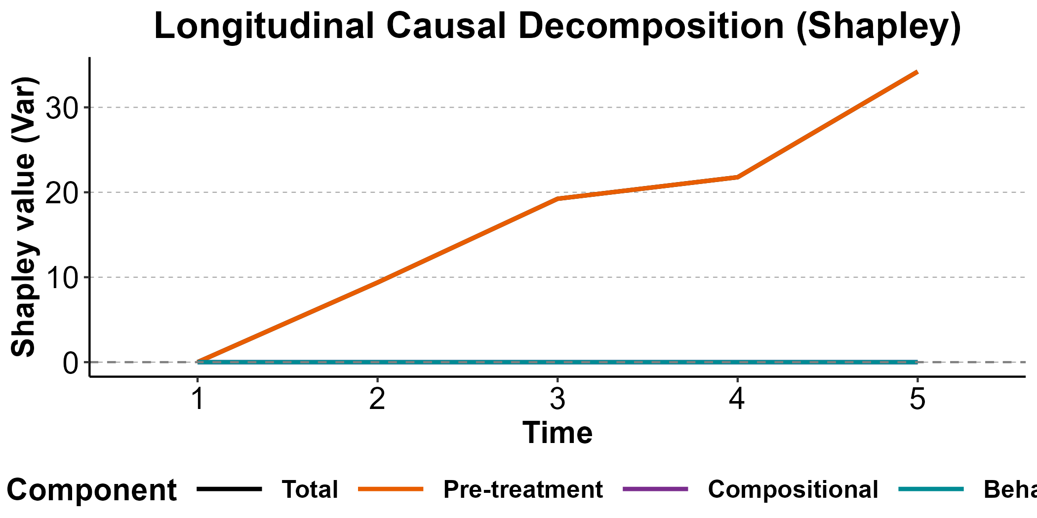

The type = "shapley" plot shows the Shapley-averaged values with ribbons indicating the range across orderings — useful for assessing ordering dependence:

plot(result_shapley, type = "shapley")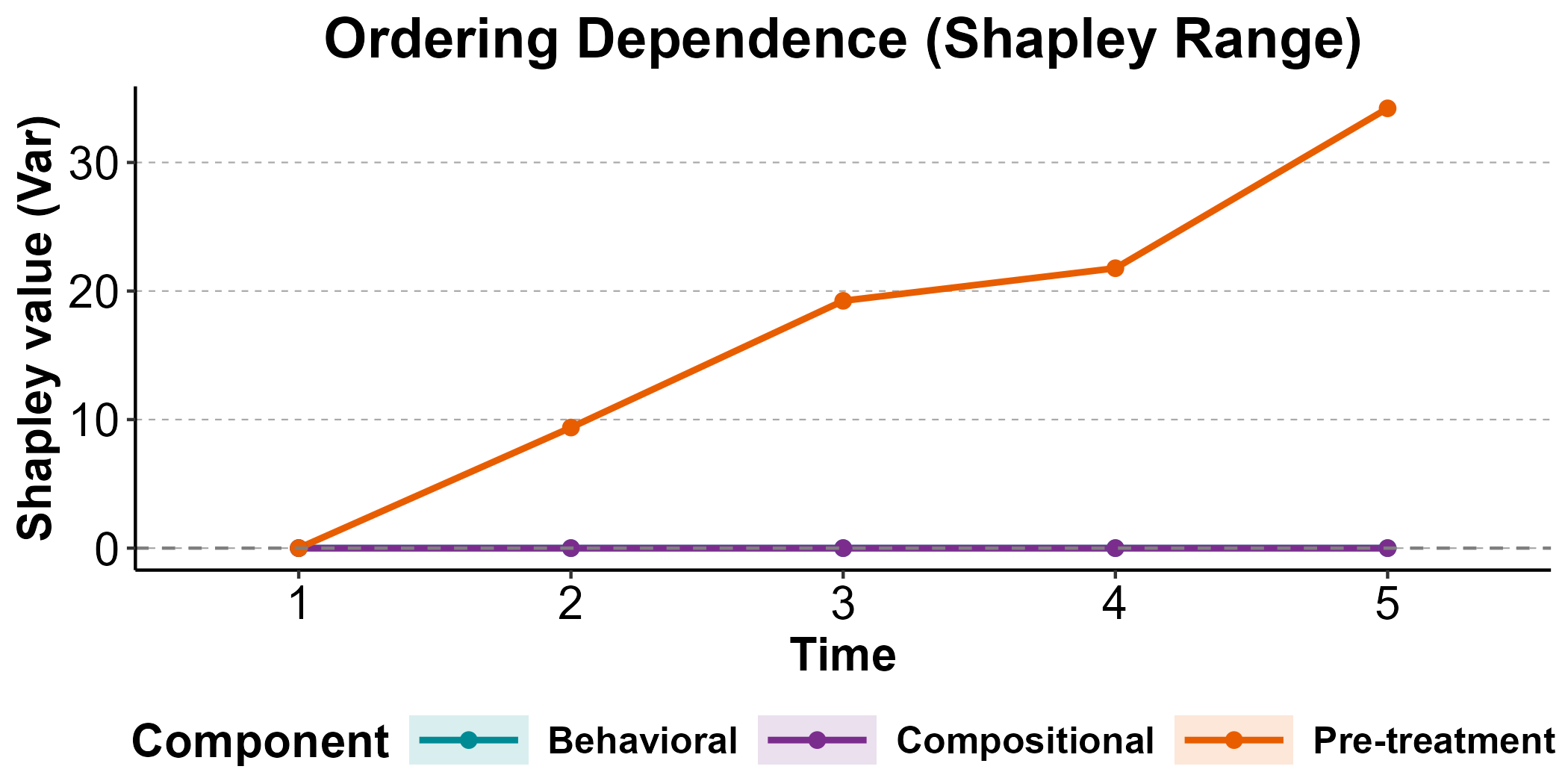

Treatment effect parameters over time

The type = "treat.params" plot shows the estimated treatment effect parameters ( $\beta$ and $\lambda$ ) by group over time:

plot(result_shapley, type = "treat.params")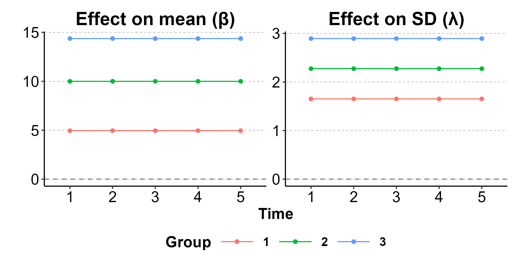

Predicted outcomes over time

The type = "outcome.params" plot compares predicted group-level means and standard deviations under control versus treatment over time:

plot(result_shapley, type = "outcome.params")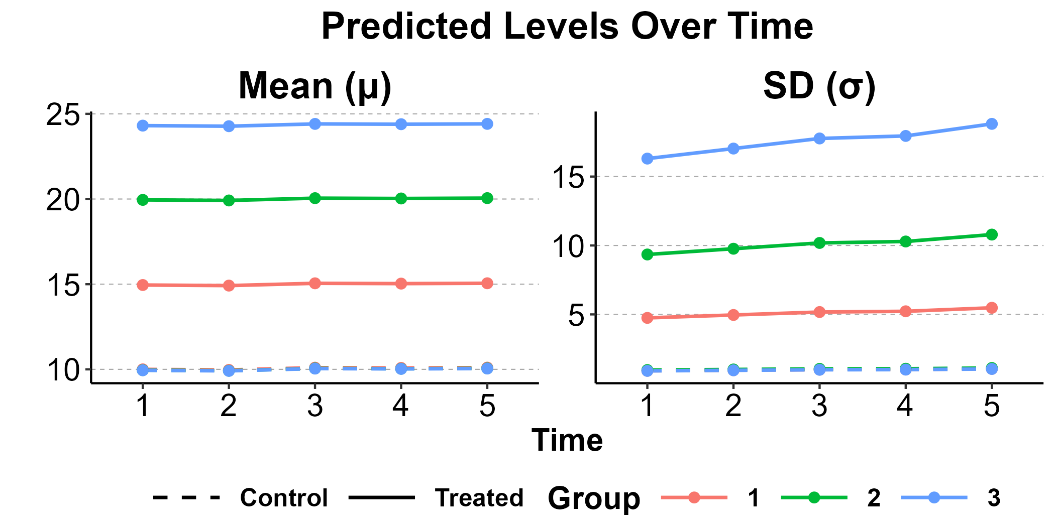

Predicted distributions

The type = "treat" plot shows predicted treatment effect distributions. When time is specified, it shows per-group distributions at that time point. When time = NULL (default), it shows pi-weighted marginal distributions across all time points. Use type = "outcome" for predicted outcome distributions:

plot(result_shapley, type = "treat", time = 3)

plot(result_shapley, type = "treat")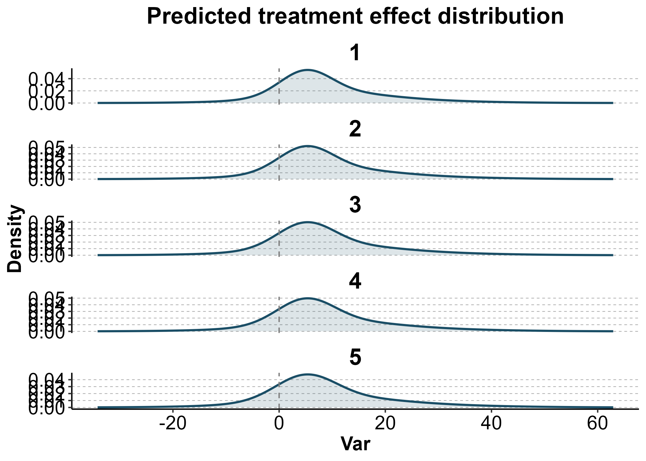

Counterfactual reference (causal)

Just as the descriptive decomposition supports a counterfactual baseline, the causal decomposition can blend user-provided counterfactual parameters with model-estimated parameters from data. This answers questions like: “How did treatment effects on inequality evolve relative to a hypothetical baseline?”

Provide an ineqx_params object (with causal columns mu0, sigma0, beta, lambda) together with treat, formula_mu, and formula_sigma. The function fits a GAMLSS model on the data, then blends the model-estimated parameters with your counterfactual scenarios.

You can specify counterfactual parameters at multiple time points. Periods covered by your params override the model estimates, while remaining periods are estimated from data. Here we place two counterfactual scenarios — one at the beginning (time 0: no treatment effect) and one in the middle (time 3: moderate, uniform treatment effect) — with data-estimated periods in between:

# Two counterfactual scenarios at time 0 and time 3
cf_ref <- ineqx_params(
  data = data.frame(
    group  = rep(1:3, 2),
    time   = rep(c(0, 3), each = 3),
    pi     = 1/3,
    mu0    = 10,
    sigma0 = 1,
    # time 0: no treatment effect
    # time 3: moderate uniform treatment effect
    beta   = c(0, 0, 0, 5, 5, 5),
    lambda = c(0, 0, 0, 1, 1, 1)
  )
)

result_blend <- ineqx(
  y             = "inc",
  treat         = "x",
  group         = "group",
  time          = "year",
  params        = cf_ref,
  ref           = 0,
  formula_mu    = ~ x * factor(group) + factor(year),
  formula_sigma = ~ x * factor(group) + factor(year),
  se            = "none",
  data          = incdat
)
#> GAMLSS-RS iteration 1: Global Deviance = 17539.56 
#> GAMLSS-RS iteration 2: Global Deviance = 16626.77 
#> GAMLSS-RS iteration 3: Global Deviance = 16626.49 
#> GAMLSS-RS iteration 4: Global Deviance = 16626.49

print(result_blend)
#> Longitudinal causal variance decomposition
#> Inequality measure: Var 
#> Reference period: 0 
#> Ordering: Shapley (averaged across all 6 orderings)
#> 
#> Treatment effect on variance by time:
#> (tau_B = Var(beta) + 2Cov(mu,beta);  tau_W = E(sigma^2)*E(f) + Cov(sigma^2,f);  tau_T = tau_B + tau_W)
#> 
#>  time  Var(beta)  2Cov(mu,beta)      tau_B E(sigma2)*E(f)  Cov(sigma2,f)      tau_W      tau_T 
#>     0     0.0000         0.0000     0.0000         0.0000         0.0000     0.0000     0.0000 
#>     1    15.5392        -0.1934    15.3459       104.1931        -1.4450   102.7481   118.0939 
#>     2    15.5392        -0.1934    15.3459       113.7054        -1.5770   112.1285   127.4743 
#>     3     0.0000         0.0000     0.0000         6.3891         0.0000     6.3891     6.3891 
#>     4    15.5392        -0.1934    15.3459       126.2725        -1.7512   124.5213   139.8671 
#>     5    15.5392        -0.1934    15.3459       138.8845        -1.9262   136.9583   152.3042 
#> 
#> Decomposition of changes in group-specific treatment effects on variance relative to ref = 0:
#> 
#>   time 0: (reference)
#> 
#>   time 1:
#>     Effects on means (delta_beta):                      15.0727
#>     Effects on SDs (delta_lambda):                     124.8056
#>     Distribution of treatment (delta_pi):              -11.1188
#>       Between-group:                                     0.3671
#>       Within-group:                                    -11.4859
#>     Pre-treatment inequality (delta_pre):              -10.6655
#>       Means:                                            -0.0939
#>       Variances:                                       -10.5716
#>     Total:                                             118.0939
#> 
#>   time 2:
#>     Effects on means (delta_beta):                      15.0727
#>     Effects on SDs (delta_lambda):                     129.8247
#>     Distribution of treatment (delta_pi):              -11.7766
#>       Between-group:                                     0.3671
#>       Within-group:                                    -12.1436
#>     Pre-treatment inequality (delta_pre):               -5.6464
#>       Means:                                            -0.0939
#>       Variances:                                        -5.5525
#>     Total:                                             127.4743
#> 
#>   time 3:
#>     Effects on means (delta_beta):                       0.0000
#>     Effects on SDs (delta_lambda):                       6.3891
#>     Distribution of treatment (delta_pi):                0.0000
#>       Between-group:                                     0.0000
#>       Within-group:                                      0.0000
#>     Pre-treatment inequality (delta_pre):                0.0000
#>       Means:                                             0.0000
#>       Variances:                                         0.0000
#>     Total:                                               6.3891
#> 
#>   time 4:
#>     Effects on means (delta_beta):                      15.0727
#>     Effects on SDs (delta_lambda):                     136.4555
#>     Distribution of treatment (delta_pi):              -12.6455
#>       Between-group:                                     0.3671
#>       Within-group:                                    -13.0126
#>     Pre-treatment inequality (delta_pre):                0.9844
#>       Means:                                            -0.0939
#>       Variances:                                         1.0783
#>     Total:                                             139.8671
#> 
#>   time 5:
#>     Effects on means (delta_beta):                      15.0727
#>     Effects on SDs (delta_lambda):                     143.1101
#>     Distribution of treatment (delta_pi):              -13.5176
#>       Between-group:                                     0.3671
#>       Within-group:                                    -13.8846
#>     Pre-treatment inequality (delta_pre):                7.6390
#>       Means:                                            -0.0939
#>       Variances:                                         7.7329
#>     Total:                                             152.3042

Time 0 and time 3 use the counterfactual parameters; times 1, 2, 4, and 5 are estimated from data via GAMLSS. The longitudinal decomposition shows how treatment effects on inequality evolved across all periods relative to the reference (time 0).

Note: delta method SEs are not available for blended parameters. Use boot_config() for bootstrap SEs if needed.

Comparing scenarios

The compare() function stacks multiple ineqx results for side-by-side comparison. This is useful for contrasting an observed decomposition with one or more counterfactual baselines:

comp <- compare(Observed = result_shapley, Counterfactual = result_blend)
#> Warning in compare(Observed = result_shapley, Counterfactual = result_blend):
#> Objects have different reference periods: 1, 0. Using ref = 1
print(comp)
#> Comparison of 2 scenarios (ineqx_causal_longit, Var)
#> Reference: 1 
#> Scenarios: Observed, Counterfactual 
#> 
#> Decomposition by time and scenario:
#>  time     component Observed Counterfactual
#>     0    behavioral       NA         0.0000
#>     0 compositional       NA         0.0000
#>     0    delta_beta       NA         0.0000
#>     0  delta_lambda       NA         0.0000
#>     0      delta_mu       NA         0.0000
#>     0    delta_pi_b       NA         0.0000
#>     0    delta_pi_w       NA         0.0000
#>     0   delta_sigma       NA         0.0000
#>     0  pretreatment       NA         0.0000
#>     1    behavioral   0.0000       139.8783
#>     1 compositional   0.0000       -11.1188
#>     1    delta_beta   0.0000        15.0727
#>     1  delta_lambda   0.0000       124.8056
#>     1      delta_mu   0.0000        -0.0939
#>     1    delta_pi_b   0.0000         0.3671
#>     1    delta_pi_w   0.0000       -11.4859
#>     1   delta_sigma   0.0000       -10.5716
#>     1  pretreatment   0.0000       -10.6655
#>     2    behavioral   0.0000       144.8974
#>     2 compositional   0.0000       -11.7766
#>     2    delta_beta   0.0000        15.0727
#>     2  delta_lambda   0.0000       129.8247
#>     2      delta_mu   0.0000        -0.0939
#>     2    delta_pi_b   0.0000         0.3671
#>     2    delta_pi_w   0.0000       -12.1436
#>     2   delta_sigma   9.3804        -5.5525
#>     2  pretreatment   9.3804        -5.6464
#>     3    behavioral   0.0000         6.3891
#>     3 compositional   0.0000         0.0000
#>     3    delta_beta   0.0000         0.0000
#>     3  delta_lambda   0.0000         6.3891
#>     3      delta_mu   0.0000         0.0000
#>     3    delta_pi_b   0.0000         0.0000
#>     3    delta_pi_w   0.0000         0.0000
#>     3   delta_sigma  19.2373         0.0000
#>     3  pretreatment  19.2373         0.0000
#>     4    behavioral   0.0000       151.5282
#>     4 compositional   0.0000       -12.6455
#>     4    delta_beta   0.0000        15.0727
#>     4  delta_lambda   0.0000       136.4555
#>     4      delta_mu   0.0000        -0.0939
#>     4    delta_pi_b   0.0000         0.3671
#>     4    delta_pi_w   0.0000       -13.0126
#>     4   delta_sigma  21.7732         1.0783
#>     4  pretreatment  21.7732         0.9844
#>     5    behavioral   0.0000       158.1828
#>     5 compositional   0.0000       -13.5176
#>     5    delta_beta   0.0000        15.0727
#>     5  delta_lambda   0.0000       143.1101
#>     5      delta_mu   0.0000        -0.0939
#>     5    delta_pi_b   0.0000         0.3671
#>     5    delta_pi_w   0.0000       -13.8846
#>     5   delta_sigma  34.2102         7.7329
#>     5  pretreatment  34.2102         7.6390

The default type = "decomp" plot uses color for the decomposition component and linetype for the scenario:

plot(comp, type = "decomp")

Use show to display individual sub-components:

plot(comp, type = "decomp",
     show = c("delta_beta", "delta_lambda", "delta_pi_b",
              "delta_pi_w", "delta_mu", "delta_sigma"))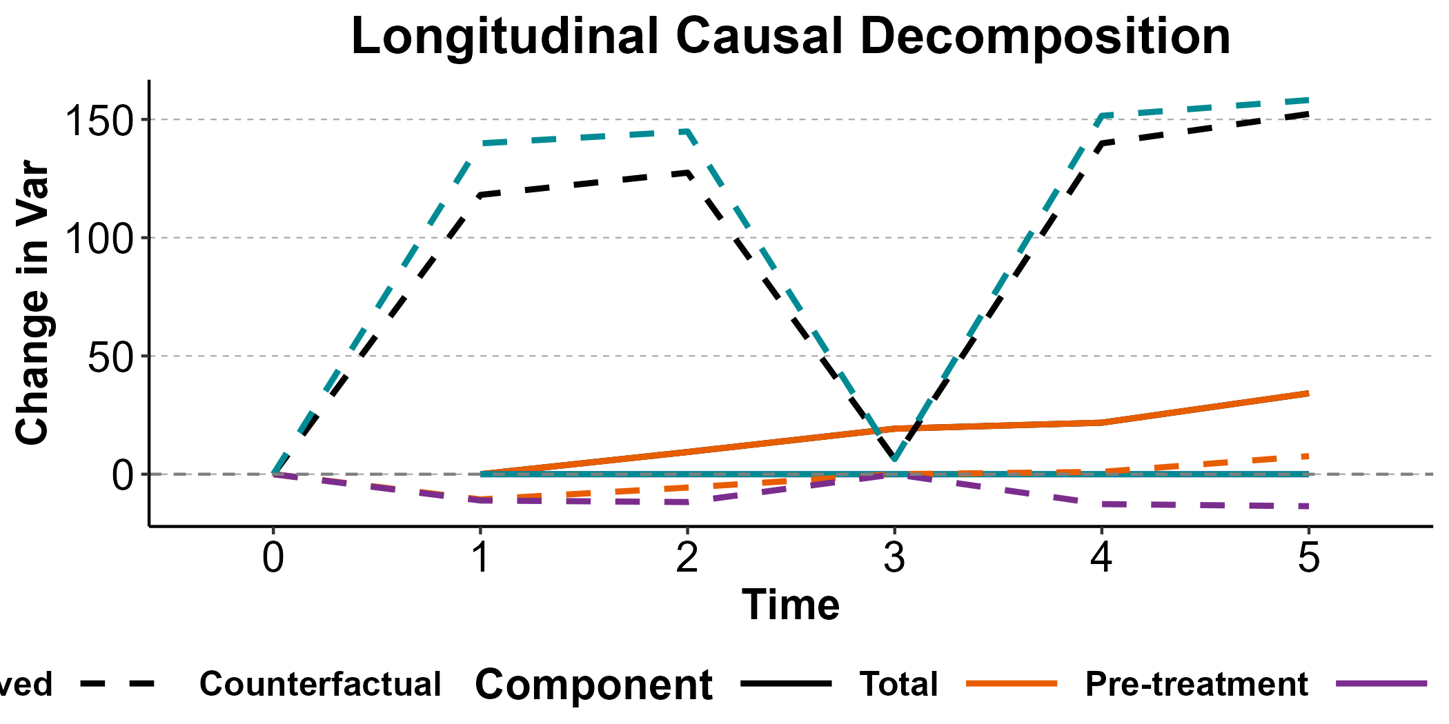

The type = "wibe" plot compares within/between treatment effect levels across scenarios:

plot(comp, type = "wibe")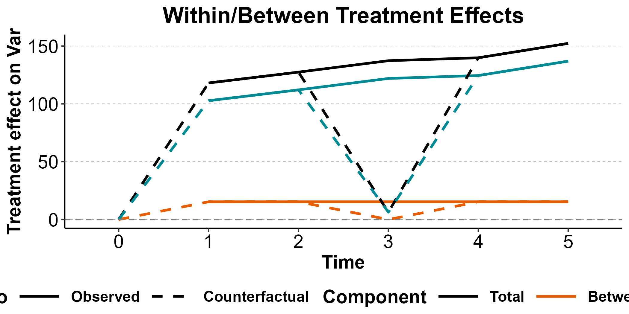

The underlying stacked data is accessible via comp$data.

3. Using an external GAMLSS model

If you want full control over the model specification (e.g., different distributions, random effects, custom controls), fit a gamlss model yourself and pass it to ineqx_params():

library(gamlss)
#> Warning: package 'gamlss' was built under R version 4.5.2
#> Warning: package 'gamlss.data' was built under R version 4.5.2
#> Warning: package 'gamlss.dist' was built under R version 4.5.2
#> Warning: package 'nlme' was built under R version 4.5.2

# Fit your own GAMLSS
my_model <- gamlss(
  formula       = inc ~ x * factor(group) + factor(t),
  sigma.formula = ~ x * factor(group) + factor(t),
  data          = incdat,
  family        = NO(),
  trace         = FALSE
)

# Extract parameters
params_ext <- ineqx_params(
  model = my_model,
  data  = incdat,
  treat = "x",
  group = "group",
  vcov  = TRUE
)

print(params_ext)
#> ineqx_params object
#>   Type: cross_sectional 
#>   Inequality measure: Var 
#>   Groups (3): 1, 2, 3
#> 
#> Group-level parameters:
#>    group     pi   mu0 sigma0   beta  lambda
#>        1 0.4737 13.87  4.191 0.1415 -0.3171
#>        2 0.2632 13.82  4.373 0.3946  0.2629
#>        3 0.2632 13.84  4.230 0.6273  0.9472
#> 
#> vcov: 12x12

# Decompose
ineqx(y="inc", group = "group", params = params_ext, data = incdat)
#> Cross-sectional causal variance decomposition
#> Inequality measure: Var 
#> SEs via delta method
#> 
#> Treatment effect on outcome variance:
#>     Var[Y | T = 0]:                         18.0601  (SE = 1.2547)
#>     Var[Y | T = 1]:                         44.2609  (SE = 2.0622)
#>     Total effect (tau_T):                   26.2008  (SE = 2.4139)
#>       Between-group (tau_B):                 0.0347  (SE = 0.0262)
#>       Within-group (tau_W):                 26.1662  (SE = 2.4138)
#>       -> Wald test H0: lambda = 0: chi2(3) = 501.2301, p < 0.0001
#>          Significant: evidence of treatment effect heterogeneity
#> 
#> Between-group sub-components:
#>     Var_pi(beta):                            0.0412  (SE = 0.0397)
#>     2*Cov_pi(mu0, beta):                    -0.0065  (SE = 0.0321)
#> 
#> Within-group sub-components:
#>     mean(sigma0^2) * mean(f):               26.1136  (SE = 2.8073)
#>     Cov_pi(sigma0^2, f):                     0.0526  (SE = 2.5861)

Manual parameter specification

You can also construct ineqx_params by hand — useful for simulation studies, sensitivity analyses, or replicating results from other software:

params_manual <- ineqx_params(
  data = data.frame(
    group  = c("low", "mid", "high"),
    pi     = c(0.4, 0.35, 0.25),
    mu0    = c(300, 600, 1200),
    sigma0 = c(100, 200, 500),
    beta   = c(50, 80, 120),
    lambda = c(-0.05, -0.10, -0.15)
  ),
  ystat = "Var"
)

ineqx(y="inc", group = "group", params = params_manual,
      se = "none", data = incdat)
#> Computing decomposition...
#> Finished.
#> Cross-sectional causal variance decomposition
#> Inequality measure: Var 
#> 
#> Treatment effect on outcome variance:
#>     Var[Y | T = 0]:                      205600.0000
#>     Var[Y | T = 1]:                      206558.7190
#>     Total effect (tau_T):                  958.7190
#>       Between-group (tau_B):             20076.0000
#>       Within-group (tau_W):              -19117.2810
#> 
#> Between-group sub-components:
#>     Var_pi(beta):                          756.0000
#>     2*Cov_pi(mu0, beta):                 19320.0000
#> 
#> Within-group sub-components:
#>     mean(sigma0^2) * mean(f):            -13387.5295
#>     Cov_pi(sigma0^2, f):                 -5729.7515

Summary

Workflow	Call	Input
Descriptive	`ineqx(y, group, data=...)`	Raw data
Descriptive (counterfactual ref)	`ineqx_params(data=...)` then `ineqx(y, group, params=..., data=...)`	Reference params + raw data
Causal (integrated)	`ineqx(y, treat, group, formula_mu=..., data=...)`	Raw data + treatment
Causal (counterfactual ref)	`ineqx_params(data=...)` then `ineqx(y, treat, group, params=..., formula_mu=..., data=...)`	Reference params + raw data + treatment
Causal (external model)	`ineqx_params(model=...)` then `ineqx(y, group, params=..., data=...)`	Fitted gamlss
Causal (manual)	`ineqx_params(data=...)` then `ineqx(y, group, params=..., data=...)`	Parameter data.frame

For details on the methodology, see vignette("model"). For more examples, see vignette("examples").